NEMO Example

For this example, the NEMO output files have already been saved as netCDF with the right coordinate names. The xorca package is designed to open NEMO datasets so they are understandable by xgcm. The xnemogcm does a similar work on idealized configurations.

Below are some example of how to make calculations using xgcm.

First we import xarray and xgcm:

import xarray as xr
import numpy as np
import xgcm
from matplotlib import pyplot as plt
%matplotlib inline
plt.rcParams['figure.figsize'] = (6,10)

Now we open the NEMO example dataset, from the BASIN configuration. The ds dataset contains the variables data (e.g. temperature, velocities) while the domcfg dataset contains the grid data (position, scale factor, etc).

We get a dataset produced for the purpose of this documentation . In this dataset, we have not outputed the vertical scale factors in the file_def_nemo-oce.xml to save space. In a real case, the scale factors need to be saved to use properly the “thickness weighted” variables. The domcfg dataset has also been filtered to remove many unused variables in this notebook (e.g. umask).

# download the data
import urllib.request
import shutil

url = 'https://zenodo.org/record/3736803/files/'
file_name_domcfg = 'xnemogcm.domcfg.nc'
with urllib.request.urlopen(url + file_name_domcfg) as response, open(file_name_domcfg, 'wb') as out_file:
    shutil.copyfileobj(response, out_file)
file_name_basin = 'xnemogcm.nemo.nc'
with urllib.request.urlopen(url + file_name_basin) as response, open(file_name_basin, 'wb') as out_file:
    shutil.copyfileobj(response, out_file)

# open the data
domcfg = xr.open_dataset(file_name_domcfg)
ds = xr.open_dataset(file_name_basin)

Add the vertical scale factors to ds (output of the model in real cases):

points = ['t', 'u', 'v', 'f', 'w']
for point in points:
    ds[f"e3{point}"] = domcfg[f"e3{point}_0"]

print('\n domcfg \n', domcfg)
print('\n ds \n', ds)

 domcfg
 <xarray.Dataset>
Dimensions:    (x_c: 20, x_f: 20, y_c: 40, y_f: 40, z_c: 36, z_f: 36)
Coordinates:
  * x_c        (x_c) int64 0 1 2 3 4 5 6 7 8 9 10 11 12 13 14 15 16 17 18 19
  * y_c        (y_c) int64 0 1 2 3 4 5 6 7 8 9 ... 30 31 32 33 34 35 36 37 38 39
  * x_f        (x_f) float64 0.5 1.5 2.5 3.5 4.5 ... 15.5 16.5 17.5 18.5 19.5
  * y_f        (y_f) float64 0.5 1.5 2.5 3.5 4.5 ... 35.5 36.5 37.5 38.5 39.5
  * z_c        (z_c) float32 5.0 15.0 25.0 35.0 ... 3.38e+03 3.787e+03 4.22e+03
  * z_f        (z_f) float32 4.5 14.5 24.5 ... 3.379e+03 3.786e+03 4.219e+03
Data variables:
    glamt      (y_c, x_c) float64 ...
    glamf      (y_f, x_f) float64 ...
    gphit      (y_c, x_c) float64 ...
    gphif      (y_f, x_f) float64 ...
    e1t        (y_c, x_c) float64 ...
    e1u        (y_c, x_f) float64 ...
    e1v        (y_f, x_c) float64 ...
    e1f        (y_f, x_f) float64 ...
    e2t        (y_c, x_c) float64 ...
    e2u        (y_c, x_f) float64 ...
    e2v        (y_f, x_c) float64 ...
    e2f        (y_f, x_f) float64 ...
    e3t_0      (z_c, y_c, x_c) float64 ...
    e3u_0      (z_c, y_c, x_f) float64 ...
    e3v_0      (z_c, y_f, x_c) float64 ...
    e3f_0      (z_c, y_f, x_f) float64 ...
    e3w_0      (z_f, y_c, x_c) float64 ...
    ht_0       (y_c, x_c) float64 ...
    fmaskutil  (y_f, x_f) float64 ...
Attributes:
    DOMAIN_number_total:     1
    DOMAIN_number:           1
    DOMAIN_dimensions_ids:   [1 2]
    DOMAIN_size_global:      [20 40]
    DOMAIN_size_local:       [20 40]
    DOMAIN_position_first:   [1 1]
    DOMAIN_position_last:    [20 40]
    DOMAIN_halo_size_start:  [0 0]
    DOMAIN_halo_size_end:    [0 0]
    DOMAIN_type:             BOX
    nn_cfg:                  2
    cn_cfg:                  BASIN

 ds
 <xarray.Dataset>
Dimensions:        (axis_nbounds: 2, t: 1, x_c: 20, x_f: 20, y_c: 40, y_f: 40, z_c: 36, z_f: 36)
Coordinates:
  * z_f            (z_f) float32 4.5 14.5 24.5 ... 3.379e+03 3.786e+03 4.219e+03
  * t              (t) object 1050-07-01 00:00:00
  * x_c            (x_c) int64 0 1 2 3 4 5 6 7 8 9 10 11 12 13 14 15 16 17 18 19
  * y_c            (y_c) int64 0 1 2 3 4 5 6 7 8 ... 31 32 33 34 35 36 37 38 39
  * z_c            (z_c) float32 5.0 15.0 25.0 ... 3.38e+03 3.787e+03 4.22e+03
  * x_f            (x_f) float64 0.5 1.5 2.5 3.5 4.5 ... 16.5 17.5 18.5 19.5
  * y_f            (y_f) float64 0.5 1.5 2.5 3.5 4.5 ... 36.5 37.5 38.5 39.5
Dimensions without coordinates: axis_nbounds
Data variables:
    depthw_bounds  (z_f, axis_nbounds) float32 ...
    t_bounds       (t, axis_nbounds) object ...
    woce           (t, z_f, y_c, x_c) float64 ...
    deptht_bounds  (z_c, axis_nbounds) float32 ...
    thetao         (t, z_c, y_c, x_c) float64 ...
    so             (t, z_c, y_c, x_c) float64 ...
    tos            (t, y_c, x_c) float64 ...
    zos            (t, y_c, x_c) float64 ...
    depthu_bounds  (z_c, axis_nbounds) float32 ...
    uos            (t, y_c, x_f) float64 ...
    uo             (t, z_c, y_c, x_f) float64 ...
    depthv_bounds  (z_c, axis_nbounds) float32 ...
    vos            (t, y_f, x_c) float64 ...
    vo             (t, z_c, y_f, x_c) float64 ...
    e3t            (z_c, y_c, x_c) float64 ...
    e3u            (z_c, y_c, x_f) float64 ...
    e3v            (z_c, y_f, x_c) float64 ...
    e3f            (z_c, y_f, x_f) float64 ...
    e3w            (z_f, y_c, x_c) float64 ...
Attributes:
    name:         NEMO dataset
    description:  Ocean grid variables, set on the proper positions
    title:        Ocean grid variables

In the coordinates, the *_c* suffix means center while the *_f* suffix means face. Thus the (x_c, y_c, z_c) point is the T point, the (x_c, y_f, z_c) is the V point, etc.

Geometry of the basin

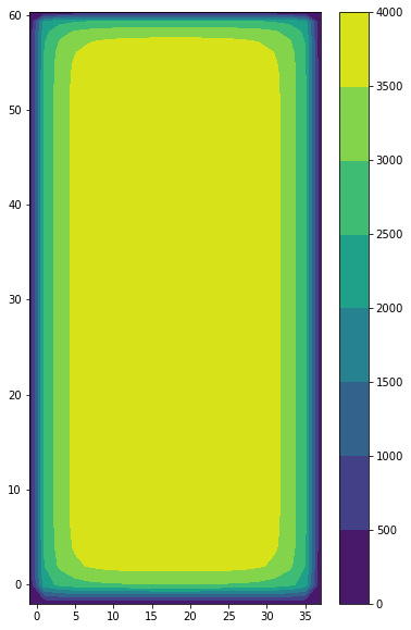
The geometry of the simulation is a closed basin, with a bottom bathymetry, going from 2000 m at the coasts, to 4000 m in the interior of the basin. Terrain following coordinates are used and the free surface is linear (fixed vertical levels). A 2 degrees Mercator grid is used.

plt.contourf(domcfg.glamt, domcfg.gphit, domcfg.ht_0)
plt.colorbar()

<matplotlib.colorbar.Colorbar at 0x7f24766cc220>

Creating the grid object

Next we create a Grid object from the dataset. All the axes are here non-periodic. The metrics dict contains the scale factors.

metrics = {
    ('X',): ['e1t', 'e1u', 'e1v', 'e1f'], # X distances
    ('Y',): ['e2t', 'e2u', 'e2v', 'e2f'], # Y distances
    ('Z',): ['e3t_0', 'e3u_0', 'e3v_0', 'e3f_0', 'e3w_0'], # Z distances
    #('X', 'Y'): [] # Areas TODO
}
grid = xgcm.Grid(domcfg, metrics=metrics, periodic=False)
print(grid)

<xgcm.Grid>
Z Axis (not periodic, boundary=None):
  * center   z_c --> left
  * left     z_f --> center
X Axis (not periodic, boundary=None):
  * center   x_c --> right
  * right    x_f --> center
Y Axis (not periodic, boundary=None):
  * center   y_c --> right
  * right    y_f --> center

We see that xgcm identified three different axes: X (longitude), Y (latitude), Z (depth).

Computation examples

Horizontal gradient of SST

We will compute the horizontal component of the gradient of SST in the longitude direction as a first example to understand the logic behind the xgcm grids.

We want to compute \(\frac{\partial SST}{\partial x}\). The SST is the variable tos (Temperature Ocean Surface) in our dataset.

In discrete form, using the NEMO notation, the derivative becomes [1]

\[\frac{\partial SST}{\partial x} = \frac{1}{e_{1u}} \delta_{i+1/2} SST = \frac{1}{e_{1u}} (SST_{i+1} - SST_i) \ .\]

The last T point is an earth point here, such as the 2 last U points: we set up the boundary argument to ‘fill’ and the fill value to zero (this value does not play an important role here, as we fill earth points).

The gradient is first computed with the diff function and then with the derivative function, the result is the same as the derivative function is aware of which scale factor to use.

---

[1] NEMO book v4.0.1, pp 22

grad_T_lon0 = grid.diff(ds.tos, axis='X', boundary='fill', fill_value=0) / domcfg.e1u
grad_T_lon1 = grid.derivative(ds.tos, axis='X', boundary='fill', fill_value=0)
print(grad_T_lon1.coords)
(grad_T_lon0 == grad_T_lon1).all()

Coordinates:
  * t        (t) object 1050-07-01 00:00:00
  * y_c      (y_c) int64 0 1 2 3 4 5 6 7 8 9 ... 30 31 32 33 34 35 36 37 38 39
  * x_f      (x_f) float64 0.5 1.5 2.5 3.5 4.5 5.5 ... 15.5 16.5 17.5 18.5 19.5

<xarray.DataArray ()>
array(True)

As expected the result of the 2 operations is the same. The position of the derivative is now on the U point.

Divergence Calculation

Here we show how to calculate the divergence of the flow. The precise details of how to do this calculation are highly model- and configuration-dependent (e.g. free-surface vs. rigid lid, etc.) In this example, the flow is incompressible, without precipitations or evaporation, with a linear free surface, satisfying the continuity equation

\[\vec{\nabla} \cdot \vec{u} = \frac{\partial u}{\partial x} + \frac{\partial v}{\partial y} + \frac{\partial w}{\partial z} = 0 \ .\]

In non-linear free surface, the divergence of \(\vec{u}\) is not 0 anymore, it is linked to the time variation of the \(e_{3}\) scale factors.

In discrete form, using NEMO notation, the equation becomes [1]

\[\vec{\nabla} \cdot \vec{u} = \frac{1}{e_{1t}e_{2t}e_{3t}} \left[ \delta_i(u \cdot e_{2u} \cdot e_{3u}) + \delta_j(v \cdot e_{1v} \cdot e_{3v}) \right] + \frac{1}{e_{3t}} \delta_k(w) \ .\]

The equation for the divergence calculation could be simplified due to the geometry of our basin, but we will keep it in the general form.

---

[1] NEMO book v4.0.1, pp 22

3d flow

We can’t use the grid.derivative function for w even if this is a simple vertical derivative: xgcm does not use the temporaly varying scale factors but the domcfg.e3t_0 initial vertical scale factors. In this simple linear free surface case, the scale factors don’t vary in time, but we will use here a more general approach.

For u and v we use the grid.diff as this is not a simple derivative, even if the horizontal scale factors are fixed in time in any case. The first T point along x is an earth point, we can use a ‘fill’ boundary with a 0 fill_value. The same argument applies along y and z.

⚠ We need to use a negative sign for the vertical derivative, as the k-axis increases with depth.

⚠ If the model is ran without linear free surface the e3 scale factors are not constant in time, we need to take the e3 from ds and not from domcfg. The data are are “thickness weighted”. To stay general, we use here the e3 scale factors from ds.

bd={'boundary':'fill', 'fill_value':0}

div_uv = grid.diff(ds.uo * domcfg.e2u * ds.e3u, 'X', **bd) / (domcfg.e1t * domcfg.e2t * ds.e3t) \
    + grid.diff(ds.vo * domcfg.e1v * ds.e3v, 'Y', **bd) / (domcfg.e1t * domcfg.e2t * ds.e3t)

div_w = - grid.diff(ds.woce, 'Z', **bd) / ds.e3t

div_uvw = div_uv + div_w
div_uvw.max()

<xarray.DataArray ()>
array(5.44218669e-19)

As expected the divergence of the flow is zero (if we neglect the truncation error).

Vertical velocity

In NEMO the vertical velocity is computed from the divergence of the horizontal velocity. In non-linear free surface, the vertical velocity can’t be computed offline because it also takes the time variations of the vertical scale factors into account. However, we are using here a linear free surface, so that

\[w(z) = \int_{bottom}^z \vec{\nabla}_h \cdot \vec{u} \, \text{d}z' = \int_{surf}^z \vec{\nabla}_h \cdot \vec{u} \, \text{d}z' - \int_{surf}^{bottom} \vec{\nabla}_h \cdot \vec{u} \, \text{d}z' \ .\]

This is written in discrete form

\[w(n) = \sum_0^n \left(\vec{\nabla}_h \cdot \vec{u}(k)\right) e_{3t}(k) - \sum_0^{n_{bot}} \left(\vec{\nabla}_h \cdot \vec{u}(k)\right) e_{3t}(k) \ .\]

We use the grid.cumsum to perform the integration, and then we remove the total integral. This is shown here with 2 methods that give the same numerical result, however the first method runs faster.

w = grid.cumsum((div_uv*ds.e3t), axis='Z', boundary='fill', fill_value=0) # integral from top
w = w - w.isel({'z_f':-1}) # now from bot

w_alt = grid.cumsum((div_uv*ds.e3t), axis='Z', boundary='fill', fill_value=0) - (div_uv*ds.e3t).sum(dim='z_c')

(w == w_alt).all()

<xarray.DataArray ()>
array(True)

Remark: the first method runs faster, indeed we perfom only once the integral.

def w1(grid, div_uv, ds):
    w = grid.cumsum((div_uv*ds.e3t), axis='Z', boundary='fill', fill_value=0) # integral from top
    return w - w.isel({'z_f':-1}) # now from bot

def w2(grid, div_uv, ds):
    return grid.cumsum((div_uv*ds.e3t), axis='Z', boundary='fill', fill_value=0) - (div_uv*ds.e3t).sum(dim='z_c')

%timeit w1(grid, div_uv, ds)
%timeit w2(grid, div_uv, ds)

4.19 ms ± 86.4 µs per loop (mean ± std. dev. of 7 runs, 100 loops each)
6.41 ms ± 232 µs per loop (mean ± std. dev. of 7 runs, 100 loops each)

We now compare the computed vertical velocity with the one outputed by the model, at the bottom of the uper grid cell.

fig, ax = plt.subplots(2, 1)
ds.woce.isel({'z_f':1}).plot(ax=ax[0])
w.isel({'z_f':1}).plot(ax=ax[1])

<matplotlib.collections.QuadMesh at 0x7f246d2efcd0>

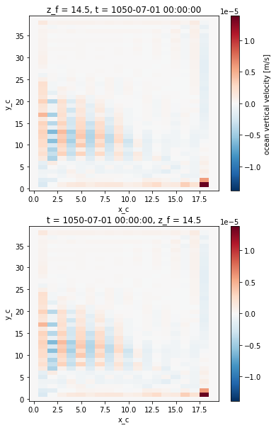
The 2 fields look similar, which is confirmed by computing the difference.

abs((w - ds.woce)).max()

<xarray.DataArray ()>
array(2.07489191e-17)

Vorticity

Here we compute more derived quantities from the velocity field.

The vertical component of the vorticity is a fundamental quantity of interest in ocean circulation theory. It is defined as

\[\zeta = \frac{\partial v}{\partial x} - \frac{\partial u}{\partial y} \ .\]

The NEMO discretization is [1]

\[\zeta = \frac{1}{e_{1f} e_{2f}} \left[\delta_{i+1/2}(v \cdot e_{2v}) - \delta_{j+1/2}(u \cdot e_{1u}) \right]\]

---

[1] NEMO book v4.0.1, pp 22

---

In xgcm, we calculate this quantity as

zeta = 1/(domcfg.e1f*domcfg.e2f) * (grid.diff(ds.vo*domcfg.e2v, 'X', **bd) - grid.diff(ds.uo*domcfg.e1u, 'Y', **bd)) * domcfg.fmaskutil
zeta.coords

Coordinates:
  * x_f      (x_f) float64 0.5 1.5 2.5 3.5 4.5 5.5 ... 15.5 16.5 17.5 18.5 19.5
  * y_f      (y_f) float64 0.5 1.5 2.5 3.5 4.5 5.5 ... 35.5 36.5 37.5 38.5 39.5
  * t        (t) object 1050-07-01 00:00:00
  * z_c      (z_c) float32 5.0 15.0 25.0 35.0 ... 3.38e+03 3.787e+03 4.22e+03

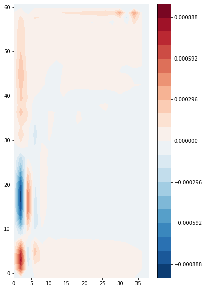
\(\zeta\) is located in the F point (x_f, y_f).

We plot the vertical integral of this quantity, i.e. the barotropic vorticity:

zeta_bt = (zeta * ds.e3f).sum(dim='z_c')
plt.contourf(
    domcfg.glamf,
    domcfg.gphif,
    zeta_bt.isel({'t':0}),
    levels=np.linspace(-abs(zeta_bt).max(), abs(zeta_bt).max(), 21),
    cmap='RdBu_r'
)
plt.colorbar()

<matplotlib.colorbar.Colorbar at 0x7f246d2acb80>

Barotropic Transport Streamfunction

We can use the barotropic velocity to calcuate the barotropic transport streamfunction, defined via

\[u_{bt} = - \frac{\partial \Psi}{\partial y} \ , \ \ v_{bt} = \frac{\partial \Psi}{\partial x} \ .\]

\[\Psi(x,y) = \int_0^x \int_{bottom}^{surface} v_{bt}(x,y) \, \text{d}z \, \text{d}x\]

We calculate this by integrating \(v_{bt}\) along the X axis using the grid object’s cumint method:

psi = grid.cumint((ds.vo*ds.e3v).sum(dim='z_c'),'X', **bd) * 1e-6
print(psi.coords)
plt.contourf(
    domcfg.glamf,
    domcfg.gphif,
    psi.isel({'t':0}),
    levels=25,
    cmap='RdBu_r'
)
plt.colorbar(label='Psi barotropic [Sv]')
plt.ylim(0,60)

Coordinates:
  * t        (t) object 1050-07-01 00:00:00
  * y_f      (y_f) float64 0.5 1.5 2.5 3.5 4.5 5.5 ... 35.5 36.5 37.5 38.5 39.5
  * x_f      (x_f) float64 0.5 1.5 2.5 3.5 4.5 5.5 ... 15.5 16.5 17.5 18.5 19.5

(0.0, 60.0)

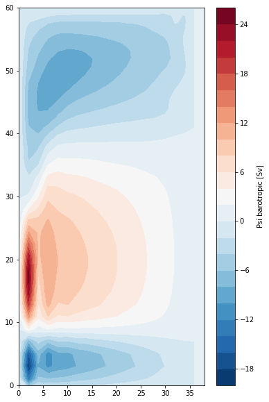
By construction, \(\psi\) is 0 at the western boundary.

Kinetic Energy

Finally, we plot the surface kinetic energy \(1/2 (u^2 + v^2)\) by interpoloting both quantities the cell center point.

# an example of calculating kinetic energy
ke = 0.5*(grid.interp((ds.uo)**2, 'X', **bd) + grid.interp((ds.vo)**2, 'Y', **bd))
ke[0,0].plot()

<matplotlib.collections.QuadMesh at 0x7f2477034e80>