Grid Topology#

Warning

The features described in this page should be considered experimental. The API is subject to change. Please report any unexpected behavior or unpleasant experiences on the github issues page

Faces and Connections#

Simple grids, as described on the Simple Grids page, consist of a single logically rectangular domain. Many modern GCMs use more complex grid topologies, consisting of multiple logically rectangular grids connected at their edges. xgcm is capable of understanding the connections between these grid faces and exchanging data between them appropriately.

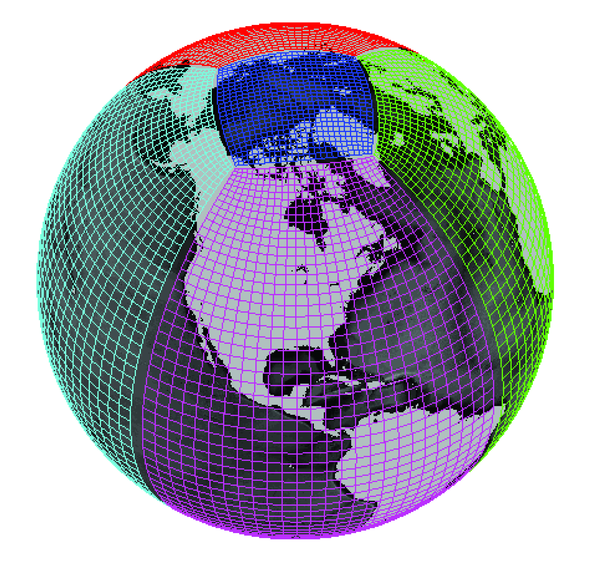
Cubed Sphre Grid — Example of a lat-lon-cap grid from the MIT General Circulation Model. Image credit Gael Forget. More information about the simulation and grid available at https://doi.org/10.5194/gmd-8-3071-2015.#

In order to construct such a complex grid topology, we need a way to tell xgcm about the connections between faces. This is accomplished via the face_connections keyword argument to the Grid constructor. Below we illustrate how this works with a series of increasingly complex examples. If you just want to get the detailed specifications for face_connections, jump down to Face Connections Spec.

Examples#

Two Connected Faces#

The simplest possible scenario is two faces connected at one side. Consider the following dataset

In [1]: import numpy as np

In [2]: import xarray as xr

In [3]: N = 25

In [4]: ds = xr.Dataset(
   ...:     {"data_c": (["face", "y", "x"], np.random.rand(2, N, N))},
   ...:     coords={
   ...:         "x": (("x",), np.arange(N), {"axis": "X"}),
   ...:         "xl": (
   ...:             ("xl"),
   ...:             np.arange(N) - 0.5,
   ...:             {"axis": "X", "c_grid_axis_shift": -0.5},
   ...:         ),
   ...:         "y": (("y",), np.arange(N), {"axis": "Y"}),
   ...:         "yl": (
   ...:             ("yl"),
   ...:             np.arange(N) - 0.5,
   ...:             {"axis": "Y", "c_grid_axis_shift": -0.5},
   ...:         ),
   ...:         "face": (("face",), [0, 1]),
   ...:     },
   ...: )
   ...: 

In [5]: ds
Out[5]: 
<xarray.Dataset>
Dimensions:  (face: 2, y: 25, x: 25, xl: 25, yl: 25)
Coordinates:
  * x        (x) int64 0 1 2 3 4 5 6 7 8 9 10 ... 15 16 17 18 19 20 21 22 23 24
  * xl       (xl) float64 -0.5 0.5 1.5 2.5 3.5 4.5 ... 19.5 20.5 21.5 22.5 23.5
  * y        (y) int64 0 1 2 3 4 5 6 7 8 9 10 ... 15 16 17 18 19 20 21 22 23 24
  * yl       (yl) float64 -0.5 0.5 1.5 2.5 3.5 4.5 ... 19.5 20.5 21.5 22.5 23.5
  * face     (face) int64 0 1
Data variables:
    data_c   (face, y, x) float64 0.9822 0.4872 0.7403 ... 0.5933 0.9538 0.6125

The dataset has two spatial axes (X and Y), plus an additional dimension face of length 2. Let’s imagine the two faces are joined in the following way:

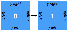
We can construct a grid that understands this connection in the following way

In [6]: import xgcm

In [7]: face_connections = {
   ...:     "face": {0: {"X": (None, (1, "X", False))}, 1: {"X": ((0, "X", False), None)}}
   ...: }
   ...: 

In [8]: grid = xgcm.Grid(ds, face_connections=face_connections)

In [9]: grid
Out[9]: 
<xgcm.Grid>
Y Axis (periodic, boundary=None):
  * center   y --> left
  * left     yl --> center
X Axis (periodic, boundary=None):
  * center   x --> left
  * left     xl --> center

The face_connections dictionary tells xgcm that face is the name of the dimension that contains the different faces. (It might have been called tile or facet or something else similar.) This dictionary say that face number 0 is connected along the X axis to nothing on the left and to face number 1 on the right. A complementary connection exists from face number 1. These connections are checked for consistency.

We can now use grid.interp() and grid.diff() to correctly interpolate and difference across the connected faces.

Two Faces with Rotated Axes#

In [10]: face_connections = {
   ....:     "face": {0: {"X": (None, (1, "Y", False))}, 1: {"Y": ((0, "X", False), None)}}
   ....: }
   ....: 

In [11]: grid = xgcm.Grid(ds, face_connections=face_connections)

In [12]: grid
Out[12]: 
<xgcm.Grid>
Y Axis (periodic, boundary=None):
  * center   y --> left
  * left     yl --> center
X Axis (periodic, boundary=None):
  * center   x --> left
  * left     xl --> center

Cubed Sphere#

A more realistic and complicated example is a cubed sphere. One possible topology for a cubed sphere grid is shown in the figure below:

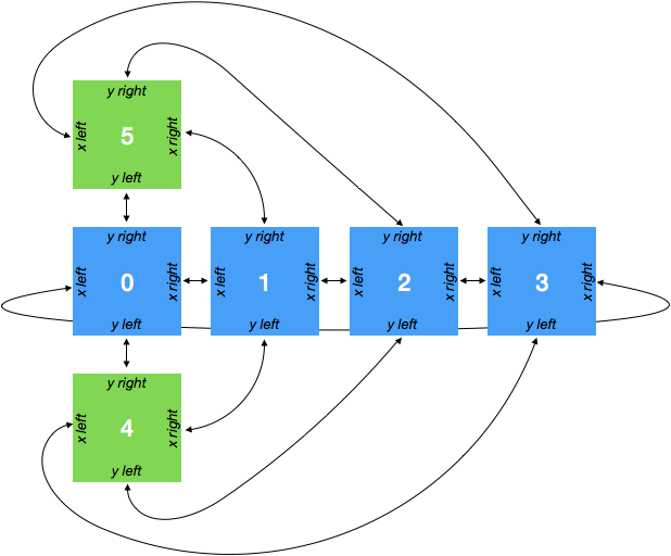
This geomtry has six faces. We can generate an xarray Dataset that has two spatial dimensions and a face dimension as follows:

In [13]: ds = xr.Dataset(
   ....:     {"data_c": (["face", "y", "x"], np.random.rand(6, N, N))},
   ....:     coords={
   ....:         "x": (("x",), np.arange(N), {"axis": "X"}),
   ....:         "xl": (
   ....:             ("xl"),
   ....:             np.arange(N) - 0.5,
   ....:             {"axis": "X", "c_grid_axis_shift": -0.5},
   ....:         ),
   ....:         "y": (("y",), np.arange(N), {"axis": "Y"}),
   ....:         "yl": (
   ....:             ("yl"),
   ....:             np.arange(N) - 0.5,
   ....:             {"axis": "Y", "c_grid_axis_shift": -0.5},
   ....:         ),
   ....:         "face": (("face",), np.arange(6)),
   ....:     },
   ....: )
   ....: 

In [14]: ds
Out[14]: 
<xarray.Dataset>
Dimensions:  (face: 6, y: 25, x: 25, xl: 25, yl: 25)
Coordinates:
  * x        (x) int64 0 1 2 3 4 5 6 7 8 9 10 ... 15 16 17 18 19 20 21 22 23 24
  * xl       (xl) float64 -0.5 0.5 1.5 2.5 3.5 4.5 ... 19.5 20.5 21.5 22.5 23.5
  * y        (y) int64 0 1 2 3 4 5 6 7 8 9 10 ... 15 16 17 18 19 20 21 22 23 24
  * yl       (yl) float64 -0.5 0.5 1.5 2.5 3.5 4.5 ... 19.5 20.5 21.5 22.5 23.5
  * face     (face) int64 0 1 2 3 4 5
Data variables:
    data_c   (face, y, x) float64 0.8968 0.1096 0.1008 ... 0.2746 0.7523 0.3658

We specify the face connections and create the Grid object as follows:

In [15]: face_connections = {
   ....:     "face": {
   ....:         0: {
   ....:             "X": ((3, "X", False), (1, "X", False)),
   ....:             "Y": ((4, "Y", False), (5, "Y", False)),
   ....:         },
   ....:         1: {
   ....:             "X": ((0, "X", False), (2, "X", False)),
   ....:             "Y": ((4, "X", False), (5, "X", True)),
   ....:         },
   ....:         2: {
   ....:             "X": ((1, "X", False), (3, "X", False)),
   ....:             "Y": ((4, "Y", True), (5, "Y", True)),
   ....:         },
   ....:         3: {
   ....:             "X": ((2, "X", False), (0, "X", False)),
   ....:             "Y": ((4, "X", True), (5, "X", False)),
   ....:         },
   ....:         4: {
   ....:             "X": ((3, "Y", True), (1, "Y", False)),
   ....:             "Y": ((2, "Y", True), (0, "Y", False)),
   ....:         },
   ....:         5: {
   ....:             "X": ((3, "Y", False), (1, "Y", True)),
   ....:             "Y": ((0, "Y", False), (2, "Y", True)),
   ....:         },
   ....:     }
   ....: }
   ....: 

In [16]: grid = xgcm.Grid(ds, face_connections=face_connections)

In [17]: grid
Out[17]: 
<xgcm.Grid>
Y Axis (periodic, boundary=None):
  * center   y --> left
  * left     yl --> center
X Axis (periodic, boundary=None):
  * center   x --> left
  * left     xl --> center

For a real-world example of how to use face connections, check out the MITgcm ECCOv4 example.

Face Connections Spec#

Because of the diversity of different model grid topologies, xgcm tries to avoid making assumptions about the nature of the connectivity between faces. It is up to the user to specify this connectivity via the face_connections dictionary. The face_connections dictionary has the following general stucture

{'<FACE DIMENSION NAME>':
    {<FACE DIMENSION VALUE>:
         {'<AXIS NAME>': (<LEFT CONNECTION>, <RIGHT CONNECTION>),
          ...}
    ...
}

<LEFT CONNECTION>> and <RIGHT CONNECTION> are either None (for no connection) or a three element tuple with the following contents

(<FACE DIMENSION VALUE>, `<AXIS NAME>`, <REVERSE CONNECTION>)

<FACE DIMENSION VALUE> tells which face this face is connected to. <AXIS NAME> tells which axis on that face is connected to this one. <REVERSE CONNECTION> is a boolean specifying whether the connection is “reversed”. A normal (non reversed) connection connects the right edge of one face to the left edge of another face. A reversed connection connects left to left, or right to right.

Note

We may consider adding standard face_connections dictionaries for common models (e.g. MITgcm, GEOS, etc.) as a convenience within xgcm. If you would like to pursue this, please open a github issue.

xgcm v0.8 documentation

Grid Topology

Contents

Grid Topology#

Faces and Connections#

Examples#

Two Connected Faces#

Two Faces with Rotated Axes#

Cubed Sphere#

Face Connections Spec#