Simple Grids#

General Concepts#

Most finite volume ocean models use Arakawa Grids, in which different variables are offset from one another and situated at different locations with respect to the cell center and edge points. As an example, we will consider C-grid geometry. As illustrated in the figure below, C-grids place scalars (such as temperature) at the cell center and vector components (such as velocity) at the cell faces. This type of grid is widely used because of its favorable conservation properties.

C-grid Geometry — Layout of variables with respect to cell centers and edges in a C-grid ocean model. Image from the pycomodo project.#

These grids present a dilemma for the xarray data model. The u and t points in the example above are located at different points along the x-axis, meaning they can’t be represented using a single coordinate. But they are clearly related and can be transformed via well defined interpolation and difference operators. One goal of xgcm is to provide these interpolation and difference operators.

We use MITgcm notation to denote the basic operators that transform between grid points. The difference operator is defined as

\[\delta_i \Phi = \Phi_{i+1/2} - \Phi_{i-1/2}\]

where \(\Phi\) is any variable and i represents the grid index. The other basic operator is interpolation, defined as

\[\overline{\Phi} = (\Phi_{i+1/2} + \Phi_{i-1/2})/2\]

Both operators return a variable that is shifted by half a gridpoint with respect to the input variable. With these two operators, the entire suite of finite volume vector calculus operations can be represented.

An important consideration for both interpolation and difference operators is boundary conditions. xgcm currently supports periodic, Dirichlet, and Neumann boundary conditions, although the latter two are limited to simple cases, see Boundary Conditions.

The inverse of differentiation is integration. For finite volume grids, the inverse of the difference operator is a discrete cumulative sum. xgcm also provides a grid-aware version of the cumsum operator.

Axes and Positions#

A fundamental concept in xgcm is the notion of an “axis”. An axis is a group of coordinates that all lie along the same physical dimension but describe different positions relative to a grid cell. There are currently five possible positions supported by xgcm.

center
The variable values are located at the cell center.

left
The variable values are located at the left (i.e. lower) face of the cell.

right
The variable values are located at the right (i.e. upper) face of the cell.

inner
The variable values are located on the cell faces, excluding both outer boundaries.

outer
The variable values are located on the cell faces, including both outer boundaries.

The first three (center, left, and right) all have the same length along the axis dimension, while inner has one fewer point and outer has one extra point. These positions are visualized in the figure below.

axis positions — The different possible positions of a variable `f` along an axis.#

xgcm represents an axis using the xgcm.Axis class.

Although it is possible to create an Axis directly, the recommended way to to use xgcm is by creating a single Grid object, containing multiple axes for each physical dimension.

Creating `Grid` Objects#

The core object in xgcm is an xgcm.Grid. A Grid object should be constructed once and then used whenever grid-aware operations are required during the course of a data analysis routine. Xgcm operates on xarray.Dataset and xarray.DataArray objects. A basic understanding of xarray data structures is therefore needed to understand xgcm.

When constructing an xgcm.Grid object, we need to pass an xarray.Dataset object containing all of the necessary coordinates for the different axes we wish to use. We also have to tell xgcm how those coordinates are related to each other, i.e. which positions they occupy along the axis. We can provide this information in two ways: manually or via dataset attributes.

Note

In most real use cases, the input dataset to create a Grid will be a come from a netCDF file generated by a GCM simulation. In this documentation, we create datasets from scratch in order to make the examples self-contained and portable.

Manually Specifying Axes#

To begin, let’s create a simple example xarray.Dataset with a single physical axis. This dataset will contain two coordinates:

x_c, which represents the cell center

x_g, which represents the left cell edge

We create it as follows.

In [1]: import xarray as xr

In [2]: import numpy as np

In [3]: ds = xr.Dataset(
   ...:     coords={
   ...:         "x_c": (
   ...:             ["x_c"],
   ...:             np.arange(1, 10),
   ...:         ),
   ...:         "x_g": (
   ...:             ["x_g"],
   ...:             np.arange(0.5, 9),
   ...:         ),
   ...:     }
   ...: )
   ...: 

In [4]: ds
Out[4]: 
<xarray.Dataset>
Dimensions:  (x_c: 9, x_g: 9)
Coordinates:
  * x_c      (x_c) int64 1 2 3 4 5 6 7 8 9
  * x_g      (x_g) float64 0.5 1.5 2.5 3.5 4.5 5.5 6.5 7.5 8.5
Data variables:
    *empty*

Note

The choice of these coordinate names (x_c and x_g) is totally arbitrary. xgcm never requires datasets to have specific variable names. Rather, the axis geometry is specified by the user or inferred through the attributes.

At this point, xarray has no idea that x_c and x_g are related to each other; they are subject to standard xarray broadcasting rules. When we create an xgcm.Grid, we need to specify that they are part of the same axis. We do this using the coords keyword argument, as follows:

In [5]: from xgcm import Grid

In [6]: grid = Grid(ds, coords={"X": {"center": "x_c", "left": "x_g"}})

In [7]: grid
Out[7]: 
<xgcm.Grid>
X Axis (periodic, boundary=None):
  * center   x_c --> left
  * left     x_g --> center

The printed information about the grid indicates that xgcm has successfully undestood the relative location of the different coordinates along the x axis. Because we did not specify the periodic keyword argument, xgcm assumed that the data is periodic along all axes. The arrows after each coordinate indicate the default shift positions for interpolation and difference operations: operating on the center coordinate (x_c) shifts to the left coordinate (x_g), and vice versa.

Detecting Axes from Dataset Attributes#

It is possible to avoid manually specifying the axis information via the coords keyword if the dataset contains specific metadata that can tell xgcm about the relationship between different coordinates. If coords is not specified, xgcm looks for this metadata in the coordinate attributes. Wherever possible, we try to follow established metadata conventions, rather than defining new metadata conventions. The two main relevant conventions are the CF Conventions, which apply broadly to Climate and Forecast datasets that follow the netCDF data model, and the COMODO conventions, which define specific attributes relevant to Arakawa grids. While the COMODO conventions were designed with C-grids in mind, we find they are general enough to support all the different Arakawa grids.

The key attribute xgcm looks for is axis. When creating a new grid, xgcm will search through the dataset dimensions looking for dimensions with the axis attribute defined. All coordinates with the same value of axis are presumed to belong to the same physical axis. To determine the positions of the different coordinates, xgcm considers both the length of the coordinate variable and the c_grid_axis_shift attribute, which determines the position of the coordinate with respect to the cell center. The only acceptable values of c_grid_axis_shift are -0.5 and 0.5. If the c_grid_axis_shift attribute attribute is absent, the coordinate is assumed to describe a cell center. The cell center coordinate is identified first; the length of other coordinates relative to the cell center coordinate is used in conjunction with c_grid_axis_shift to infer the coordinate positions, as summarized by the table below.

length	`c_grid_axis_shift`	position
n	None	center
n	-0.5	left
n	0.5	right
n-1	0.5 or -0.5	inner
n+1	0.5 or -0.5	outer

We create an xarray.Dataset with such attributes as follows:

In [8]: ds = xr.Dataset(
   ...:     coords={
   ...:         "x_c": (
   ...:             ["x_c"],
   ...:             np.arange(1, 10),
   ...:             {"axis": "X"},
   ...:         ),
   ...:         "x_g": (
   ...:             ["x_g"],
   ...:             np.arange(0.5, 9),
   ...:             {"axis": "X", "c_grid_axis_shift": -0.5},
   ...:         ),
   ...:     }
   ...: )
   ...: 

In [9]: ds
Out[9]: 
<xarray.Dataset>
Dimensions:  (x_c: 9, x_g: 9)
Coordinates:
  * x_c      (x_c) int64 1 2 3 4 5 6 7 8 9
  * x_g      (x_g) float64 0.5 1.5 2.5 3.5 4.5 5.5 6.5 7.5 8.5
Data variables:
    *empty*

(This is the same as the first example, just with additional attributes.) We can now create a Grid object from this dataset without manually specifying coords:

In [10]: grid = Grid(ds)

In [11]: grid
Out[11]: 
<xgcm.Grid>
X Axis (periodic, boundary=None):
  * center   x_c --> left
  * left     x_g --> center

We see that the resulting Grid object is the same as in the manual example.

Core Grid Operations: `diff`, `interp`, and `cumsum`#

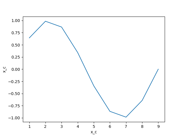
Regardless of how our Grid object was created, we can now use it to interpolate or take differences along the axis. First we create some test data:

In [12]: import matplotlib.pyplot as plt

In [13]: da = np.sin(ds.x_c * 2 * np.pi / 9)

In [14]: print(da)
<xarray.DataArray 'x_c' (x_c: 9)>
array([ 6.42787610e-01,  9.84807753e-01,  8.66025404e-01,  3.42020143e-01,
       -3.42020143e-01, -8.66025404e-01, -9.84807753e-01, -6.42787610e-01,
       -2.44929360e-16])
Coordinates:
  * x_c      (x_c) int64 1 2 3 4 5 6 7 8 9

In [15]: da.plot()
Out[15]: [<matplotlib.lines.Line2D at 0x7f102b1d0a30>]

In [16]: plt.close()

We interpolate as follows:

In [17]: da_interp = grid.interp(da, axis="X")

In [18]: da_interp
Out[18]: 
<xarray.DataArray 'x_c' (x_g: 9)>
array([ 3.21393805e-01,  8.13797681e-01,  9.25416578e-01,  6.04022774e-01,
        1.11022302e-16, -6.04022774e-01, -9.25416578e-01, -8.13797681e-01,
       -3.21393805e-01])
Coordinates:
  * x_g      (x_g) float64 0.5 1.5 2.5 3.5 4.5 5.5 6.5 7.5 8.5

We see that the output is on the x_g points rather than the original x_c points.

Warning

xgcm does not perform input validation to verify that da is compatible with grid.

The same position shift happens with a difference operation:

In [19]: da_diff = grid.diff(da, axis="X")

In [20]: da_diff
Out[20]: 
<xarray.DataArray 'x_c' (x_g: 9)>
array([ 0.64278761,  0.34202014, -0.11878235, -0.52400526, -0.68404029,
       -0.52400526, -0.11878235,  0.34202014,  0.64278761])
Coordinates:
  * x_g      (x_g) float64 0.5 1.5 2.5 3.5 4.5 5.5 6.5 7.5 8.5

We can reverse the difference operation by taking a cumsum:

In [21]: grid.cumsum(da_diff, "X")
Out[21]: 
<xarray.DataArray 'x_c' (x_c: 9)>
array([ 6.42787610e-01,  9.84807753e-01,  8.66025404e-01,  3.42020143e-01,
       -3.42020143e-01, -8.66025404e-01, -9.84807753e-01, -6.42787610e-01,
        1.11022302e-16])
Coordinates:
  * x_c      (x_c) int64 1 2 3 4 5 6 7 8 9

Which is approximately equal to the original da, modulo the numerical errors accrued due to the discretization of the data.

By default, these grid operations will drop any coordinate that are not dimensions. The keep_coords argument allow to preserve compatible coordinates. For example:

In [22]: da2 = da + xr.Dataset(coords={"y": np.arange(1, 3)})["y"]

In [23]: da2 = da2.assign_coords(h=da2.y**2)

In [24]: print(da2)
<xarray.DataArray (x_c: 9, y: 2)>
array([[1.64278761, 2.64278761],
       [1.98480775, 2.98480775],
       [1.8660254 , 2.8660254 ],
       [1.34202014, 2.34202014],
       [0.65797986, 1.65797986],
       [0.1339746 , 1.1339746 ],
       [0.01519225, 1.01519225],
       [0.35721239, 1.35721239],
       [1.        , 2.        ]])
Coordinates:
  * x_c      (x_c) int64 1 2 3 4 5 6 7 8 9
  * y        (y) int64 1 2
    h        (y) int64 1 4

In [25]: grid.interp(da2, "X", keep_coords=True)
Out[25]: 
<xarray.DataArray (x_g: 9, y: 2)>
array([[1.3213938 , 2.3213938 ],
       [1.81379768, 2.81379768],
       [1.92541658, 2.92541658],
       [1.60402277, 2.60402277],
       [1.        , 2.        ],
       [0.39597723, 1.39597723],
       [0.07458342, 1.07458342],
       [0.18620232, 1.18620232],
       [0.6786062 , 1.6786062 ]])
Coordinates:
  * x_g      (x_g) float64 0.5 1.5 2.5 3.5 4.5 5.5 6.5 7.5 8.5
Dimensions without coordinates: y

So far we have just discussed simple grids (i.e. regular grids with a single face). Xgcm can also deal with complex topologies such as cubed-sphere and lat-lon-cap. This is described in the grid_topology page.

xgcm v0.8 documentation

Simple Grids

Contents

Simple Grids#

General Concepts#

Axes and Positions#

Creating `Grid` Objects#

Manually Specifying Axes#

Detecting Axes from Dataset Attributes#

Core Grid Operations: `diff`, `interp`, and `cumsum`#

xgcm v0.8 documentation

Simple Grids

Contents

Simple Grids#

General Concepts#

Axes and Positions#

Creating Grid Objects#

Manually Specifying Axes#

Detecting Axes from Dataset Attributes#

Core Grid Operations: diff, interp, and cumsum#

Creating `Grid` Objects#

Core Grid Operations: `diff`, `interp`, and `cumsum`#