Grid Ufuncs#
Concept of a Grid Ufunc#
In short, a “grid ufunc” is a generalisation of a numpy generalized universal function to include the xGCM Axes and Positions of input and output variables.
If you are not already familiar with the concept numpy generalized universal function (hereon referred to a “numpy ufunc”),
then have a read of the linked documentation.
You will also need to understand the concept of “core dims” used in xarray.apply_ufunc.
We tell a grid ufunc about the xGCM axes information through a signature.
For example, imagine we have a function which accepts data located at the center grid positions and returns
data located at the left-hand grid positions, on the same axis.
The signature for this function would look like:
"(ax1:center)->(ax1:left)".
Grid ufuncs allow us to:
Avoid mistakes by stating that functions are only valid for data on specific grid positions,
Neatly promote numpy functions to grid-aware xarray functions,
Conveniently apply Boundary Conditions and Grid Topology,
Boost performance relative to chaining many
Grid.difforGrid.interpoperations,Immediately parallelize our operations with dask (see Parallelizing with Dask).
The signature#
The “signature” of a grid ufunc is how we tell it which input and output variables should be on which axis positions.
A simple example would be
"(ax1:center)->(ax1:left)"
The signature has two parts, one for the input variables, and one for the output variables.
The output variables live on the right of the arrow (->).
There needs to be one entry in parentheses for each variable, so in this case the signature tells use that the function accepts one input data variable and returns one output data variable. (Functions which accept a data variable in the form of a keyword-only argument are not supported.)
For each variable, the signature tells us the xgcm.Axis positions we require that variable to have,
both before and after our grid ufunc is applied.
This information is encoded in the format axis_name:position.
Each variable can be operated on along multiple axes, which are separated by a comma, e.g. (ax1:left, ax2:right).
The axis names used in the signature are dummy names: they do not have to be the same as the axis names used in your Grid object.
This allows you to write a grid ufunc that can accept axes with any name.
Therefore the signature "(ax1:center)->(ax1:left)" means all of:
“This function accepts one data variable and applies an operation over one core dimension. The input data lies on the center grid positions of the singular axis along which we will choose to apply the function. After performing its numerical operation the single return value from this function will have been shifted onto the left-hand grid positions of the same axis.”
To give you an idea of how we might use grid ufuncs here is a table of possible grid ufuncs and their corresponding signatures:
Name |
Signature |
Description |
|---|---|---|
|
|
Backward difference |
|
|
Backward interpolation |
|
|
Forward difference |
|
|
Forward interpolation |
|
|
Second order central difference |
|
|
Reduction |
|
|
Reduction of two variables |
|
|
Complex example calculating vorticity on an Arakawa U-grid in 2D |
Note
Remember the axis names in the signature are dummy names - in the example above you could apply mean_depth along
an axis not called "depth" if you wish.
The axis argument is the one which must correspond to an xgcm.Axis of the grid.
Therefore applying a grid ufunc with signature "(X:center)->()" or "(depth:center)->()" along axis='X' will
yield identical results in both cases.
Defining New Grid Ufuncs#
Let’s imagine we have a numpy function which does forward differencing along one dimension, with an implicit periodic boundary condition.
In [1]: import numpy as np
In [2]: def diff_forward(a):
   ...:     return a - np.roll(a, -1, axis=-1)
   ...:
All this function does is subtract each element of the given array from the element immediately to its right,
with the ends of the array wrapped around in a periodic fashion.
If we imagine this function acting on a variable located at the cell centers,
our Axes and Positions diagram suggests that the result would lie on the left-hand cell edges.
Therefore the signature of this function could be
"(ax1:center)->(ax1:left)".
Note
XGCM assumes the function acts along the last axis of the numpy array, which is why we have specified axis=-1 here.
There are multiple options for how to apply this numpy ufunc as a grid ufunc.
We’re going to need a grid object, and some data, so we use the same demonstration grid and dataarray that we defined when we introduced Simple Grids.
Our grid object has one Axis ("X"), which has two coordinates, on positions "center" and "left".
In [3]: import xarray as xr

In [4]: from xgcm import Grid

In [5]: ds = xr.Dataset(
   ...:     coords={
   ...:         "x_c": (
   ...:             ["x_c"],
   ...:             np.arange(1, 10),
   ...:         ),
   ...:         "x_g": (
   ...:             ["x_g"],
   ...:             np.arange(0.5, 9),
   ...:         ),
   ...:     }
   ...: )
   ...:

In [6]: grid = Grid(
   ...:     ds, coords={"X": {"center": "x_c", "left": "x_g"}}, autoparse_metadata=False
   ...: )
   ...:

In [7]: grid
Out[7]:
<xgcm.Grid>
X Axis (periodic, boundary='periodic'):
  * center   x_c --> left
  * left     x_g --> center
Our data starts on the cell centers.
In [8]: da = np.sin(ds.x_c * 2 * np.pi / 9)

In [9]: da
Out[9]:
<xarray.DataArray 'x_c' (x_c: 9)> Size: 72B
array([ 6.42787610e-01,  9.84807753e-01,  8.66025404e-01,  3.42020143e-01,
       -3.42020143e-01, -8.66025404e-01, -9.84807753e-01, -6.42787610e-01,
       -2.44929360e-16])
Coordinates:
  * x_c      (x_c) int64 72B 1 2 3 4 5 6 7 8 9
Applying directly#
The quickest option is to apply our function directly, using apply_as_grid_ufunc
In [10]: from xgcm import apply_as_grid_ufunc

In [11]: result = apply_as_grid_ufunc(
   ....:     diff_forward, da, axis=[["X"]], signature="(ax1:center)->(ax1:left)", grid=grid
   ....: )
   ....:

In [12]: result
Out[12]:
<xarray.DataArray 'x_c' (x_g: 9)> Size: 72B
array([-0.34202014,  0.11878235,  0.52400526,  0.68404029,  0.52400526,
        0.11878235, -0.34202014, -0.64278761, -0.64278761])
Coordinates:
  * x_g      (x_g) float64 72B 0.5 1.5 2.5 3.5 4.5 5.5 6.5 7.5 8.5
Here we have applied the grid ufunc to the data, along the axis "X" of the grid.
(The nested-list format of axis is to match the fact we supplied one input data variable, which only has one axis.)
The dummy axis name ax1 gets substituted by "X" during the call, so this will fail if our data does not depend on the axis we attempt to apply the ufunc along.
We can see that the result has been shifted onto the output grid positions along "X", so now lies on the left-hand cell edges.
Decorator with signature#
Alternatively you can permanently turn a numpy function into a grid ufunc by using the @as_grid_ufunc decorator.
In [13]: from xgcm import as_grid_ufunc
In [14]: @as_grid_ufunc(signature="(ax1:center)->(ax1:left)")
   ....: def diff_center_to_left(a):
   ....:     return diff_forward(a)
   ....:
Now when we call the diff_center_to_left function, it will act as if we had applied it using apply_as_grid_ufunc.
In [15]: diff_center_to_left(grid, da, axis=[["X"]])
Out[15]:
<xarray.DataArray 'x_c' (x_g: 9)> Size: 72B
array([-0.34202014,  0.11878235,  0.52400526,  0.68404029,  0.52400526,
        0.11878235, -0.34202014, -0.64278761, -0.64278761])
Coordinates:
  * x_g      (x_g) float64 72B 0.5 1.5 2.5 3.5 4.5 5.5 6.5 7.5 8.5
Notice that we still need to provide the grid and axis arguments when we call the decorated function.
Decorator with type hints#
Finally you can use type hints to specify the grid positions of the variables instead of passing a signature argument.
In [16]: from typing import Annotated
In [17]: @as_grid_ufunc()
   ....: def diff_center_to_left(
   ....:     a: Annotated[np.ndarray, "ax1:center"]
   ....: ) -> Annotated[np.ndarray, "ax1:left"]:
   ....:     return diff_forward(a)
   ....:
Again we call this decorated function, remembering to supply the grid and axis arguments
In [18]: diff_center_to_left(grid, da, axis=[["X"]])
Out[18]:
<xarray.DataArray 'x_c' (x_g: 9)> Size: 72B
array([-0.34202014,  0.11878235,  0.52400526,  0.68404029,  0.52400526,
        0.11878235, -0.34202014, -0.64278761, -0.64278761])
Coordinates:
  * x_g      (x_g) float64 72B 0.5 1.5 2.5 3.5 4.5 5.5 6.5 7.5 8.5
The signature argument is incompatible with using Annotated to annotate the types of any of the function arguments
- i.e. you cannot mix the signature approach with the type hinting approach.
Note
If you want to use type hints to specify a signature with multiple return arguments, your return value should be type hinted as a tuple of annotated hints, e.g.
Tuple[Annotated[np.ndarray, "ax1:left"], Annotated[np.ndarray, "ax1:right"]].
Boundaries and Padding#
Manually Applying Boundary Conditions#
The example differencing function we used above had an implicit periodic boundary condition, but what if we wanted to use a different boundary condition?
We’ll show this using a simple linear interpolation function. It has the same signature at the differencing function we used above, but it does not apply any specific boundary condition.
In [19]: def interp(a):
   ....:     return 0.5 * (a[..., :-1] + a[..., 1:])
   ....:
This function simply averages each element from the one on its right, but that means the resulting array is shorter by one element.
In [20]: arr = np.arange(9)

In [21]: arr
Out[21]: array([0, 1, 2, 3, 4, 5, 6, 7, 8])

In [22]: arr.shape
Out[22]: (9,)

In [23]: interpolated = interp(arr)

In [24]: interpolated
Out[24]: array([0.5, 1.5, 2.5, 3.5, 4.5, 5.5, 6.5, 7.5])

In [25]: interpolated.shape
Out[25]: (8,)
Applying a boundary condition during this operation is equivalent to choosing how to pad the original array
so that the application of interp still returns an array of the starting length.
We could do this manually - implementing a periodic boundary condition would mean first pre-pending the right-most element of the input array onto the left-hand side:
In [26]: periodically_padded_arr = np.insert(arr, 0, arr[-1])

In [27]: periodically_padded_arr
Out[27]: array([8, 0, 1, 2, 3, 4, 5, 6, 7, 8])

In [28]: interpolated_periodically = interp(periodically_padded_arr)

In [29]: interpolated_periodically.shape
Out[29]: (9,)
and implementing a constant zero-padding boundary condition would mean first pre-pending the input array with a zero:
In [30]: zero_padded_arr = np.insert(arr, 0, 0)

In [31]: zero_padded_arr
Out[31]: array([0, 0, 1, 2, 3, 4, 5, 6, 7, 8])

In [32]: interpolated_with_zero_padding = interp(zero_padded_arr)

In [33]: interpolated_with_zero_padding
Out[33]: array([0. , 0.5, 1.5, 2.5, 3.5, 4.5, 5.5, 6.5, 7.5])

In [34]: interpolated_with_zero_padding.shape
Out[34]: (9,)
In both cases the result has the same length as the original input array. We can also see that the result depends on the choice of boundary conditions.
Automatically Applying Boundary Conditions#
Doing this manually is a chore, so xgcm allows you to apply boundary conditions automatically when using grid ufuncs.
When doing the padding manually for interp, we had to add one element on the left-hand side of the `"X" axis,
so we tell xGCM to do the same thing by specifying the keyword argument boundary_width={"X": (1, 0)},
In [35]: @as_grid_ufunc(signature="(X:center)->(X:left)", boundary_width={"X": (1, 0)})
   ....: def interp_center_to_left(a):
   ....:     return interp(a)
   ....:
Now when we run our decorated function interp_center_to_left, xgcm will automatically add an extra element to the left hand side for us, before applying the operation in the function we decorated.
# Create new test data with same coordinates but linearly-spaced data
In [36]: da = da.copy(data=arr)

In [37]: interp_center_to_left(grid, da, axis=[["X"]])
Out[37]:
<xarray.DataArray 'x_c' (x_g: 9)> Size: 72B
array([4. , 0.5, 1.5, 2.5, 3.5, 4.5, 5.5, 6.5, 7.5])
Coordinates:
  * x_g      (x_g) float64 72B 0.5 1.5 2.5 3.5 4.5 5.5 6.5 7.5 8.5
Here a periodic boundary condition has been used as the default, but we can choose other boundary conditions using the boundary kwarg:
In [38]: @as_grid_ufunc(
   ....:     signature="(X:center)->(X:left)",
   ....:     boundary_width={"X": (1, 0)},
   ....:     boundary="fill",
   ....:     fill_value=0,
   ....: )
   ....: def interp_center_to_left_fill_with_zeros(a):
   ....:     return interp(a)
   ....:
In [39]: interp_center_to_left_fill_with_zeros(
   ....:     grid, da, axis=[["X"]], boundary="fill", fill_value=0
   ....: )
   ....:
Out[39]:
<xarray.DataArray 'x_c' (x_g: 9)> Size: 72B
array([0. , 0.5, 1.5, 2.5, 3.5, 4.5, 5.5, 6.5, 7.5])
Coordinates:
  * x_g      (x_g) float64 72B 0.5 1.5 2.5 3.5 4.5 5.5 6.5 7.5 8.5
We can also choose a different default boundary condition at decorator definition time, and then override it at function call time if we prefer.
In [40]: interp_center_to_left(grid, da, axis=[["X"]], boundary="fill", fill_value=0)
Out[40]:
<xarray.DataArray 'x_c' (x_g: 9)> Size: 72B
array([0. , 0.5, 1.5, 2.5, 3.5, 4.5, 5.5, 6.5, 7.5])
Coordinates:
  * x_g      (x_g) float64 72B 0.5 1.5 2.5 3.5 4.5 5.5 6.5 7.5 8.5
For more advanced examples of grid ufuncs, see the page on ufunc examples.
Metrics#
Note
Automatically supplying metrics directly to grid ufuncs is not yet implemented, but will be soon! For now, if you need a metric in your grid ufunc, simply include it as an input and pass it explicitly. To work with metrics outside of grid ufuncs see the documentation page on metrics.
Parallelizing with Dask#
The grid ufunc apparatus is designed so that if your data is chunked, it will apply your ufunc operation in a dask-efficient manner. There are two cases of interest to understand: parallelizing an operation over data chunked along a “broadcast” dimension, and over data chunked along a “core” dimension.
If you don’t know what that means then read about the concept of “core dims” used in xarray.apply_ufunc.
Parallelizing Along Broadcast Dimensions#
This case is for when your data is chunked along the dim corresponding to the axis along which you want to apply the grid ufunc. The numpy ufunc you are wrapping must be able to act on each element along that axis independently.
This case is parallelized under the hood by calling xarray.apply_ufunc.
In order to enable working with chunked arrays you must pass the kwarg dask='parallelized' to apply_as_grid_ufunc.
# Let's create some 2D data, so we have a dimension over which to broadcast
In [41]: da_2d = da.expand_dims(y=4)

# Let's also chunk it along the new "broadcast" dimension
In [42]: chunked_y = da_2d.chunk({"y": 1})

In [43]: chunked_y
Out[43]:
<xarray.DataArray 'x_c' (y: 4, x_c: 9)> Size: 288B
dask.array<xarray-<this-array>, shape=(4, 9), dtype=int64, chunksize=(1, 9), chunktype=numpy.ndarray>
Coordinates:
  * x_c      (x_c) int64 72B 1 2 3 4 5 6 7 8 9
Dimensions without coordinates: y

In [44]: result = interp_center_to_left(grid, chunked_y, axis=[["X"]], dask="parallelized")
(We could also have passed the dask kwarg to the @as_grid_ufunc decorator, and it would have been bound
to the new function in the same way that the boundary kwargs work.)
The dask graph in this case is simple, because this is an “embarrasingly parallel” problem.
result.data.visualize(optimize_graph=True)
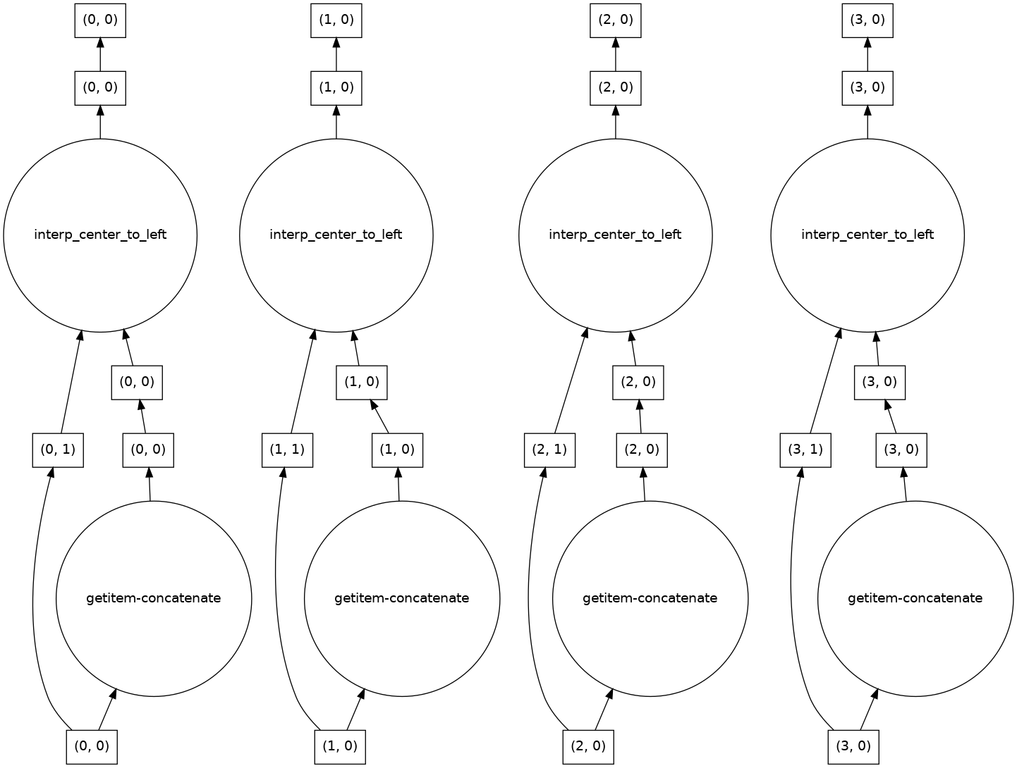
The result is as expected from padding each row independently.
In [45]: result.compute()
Out[45]:
<xarray.DataArray 'x_c' (y: 4, x_g: 9)> Size: 288B
array([[4. , 0.5, 1.5, 2.5, 3.5, 4.5, 5.5, 6.5, 7.5],
       [4. , 0.5, 1.5, 2.5, 3.5, 4.5, 5.5, 6.5, 7.5],
       [4. , 0.5, 1.5, 2.5, 3.5, 4.5, 5.5, 6.5, 7.5],
       [4. , 0.5, 1.5, 2.5, 3.5, 4.5, 5.5, 6.5, 7.5]])
Coordinates:
  * x_g      (x_g) float64 72B 0.5 1.5 2.5 3.5 4.5 5.5 6.5 7.5 8.5
Dimensions without coordinates: y
Parallelizing Along Core Dimensions#
The other case is for when your data is chunked along the axis over which you want to apply your ufunc (a “core” dimension”).
In [46]: chunked_x = da_2d.chunk({"x_c": 2})

In [47]: chunked_x
Out[47]:
<xarray.DataArray 'x_c' (y: 4, x_c: 9)> Size: 288B
dask.array<xarray-<this-array>, shape=(4, 9), dtype=int64, chunksize=(4, 2), chunktype=numpy.ndarray>
Coordinates:
  * x_c      (x_c) int64 72B 1 2 3 4 5 6 7 8 9
Dimensions without coordinates: y
XGCM can also parallelize this case, by calling dask.map_overlap.
You tell it to invoke dask.map_overlap by passing dask="parallelized" and map_overlap=True.
In [48]: result = interp_center_to_left(
   ....:     grid, chunked_x, axis=[["X"]], dask="allowed", map_overlap=True
   ....: )
   ....:
If your ufunc operates on individual chunks independently, then dask.map_blocks would have been sufficient,
but the possibility of padding boundaries means that dask.map_overlap is required.
The dask graph is more complicated, because each chunk along the core dim needs to communicate its boundary_width elements to adjacent chunks.
result.data.visualize(optimize_graph=True)
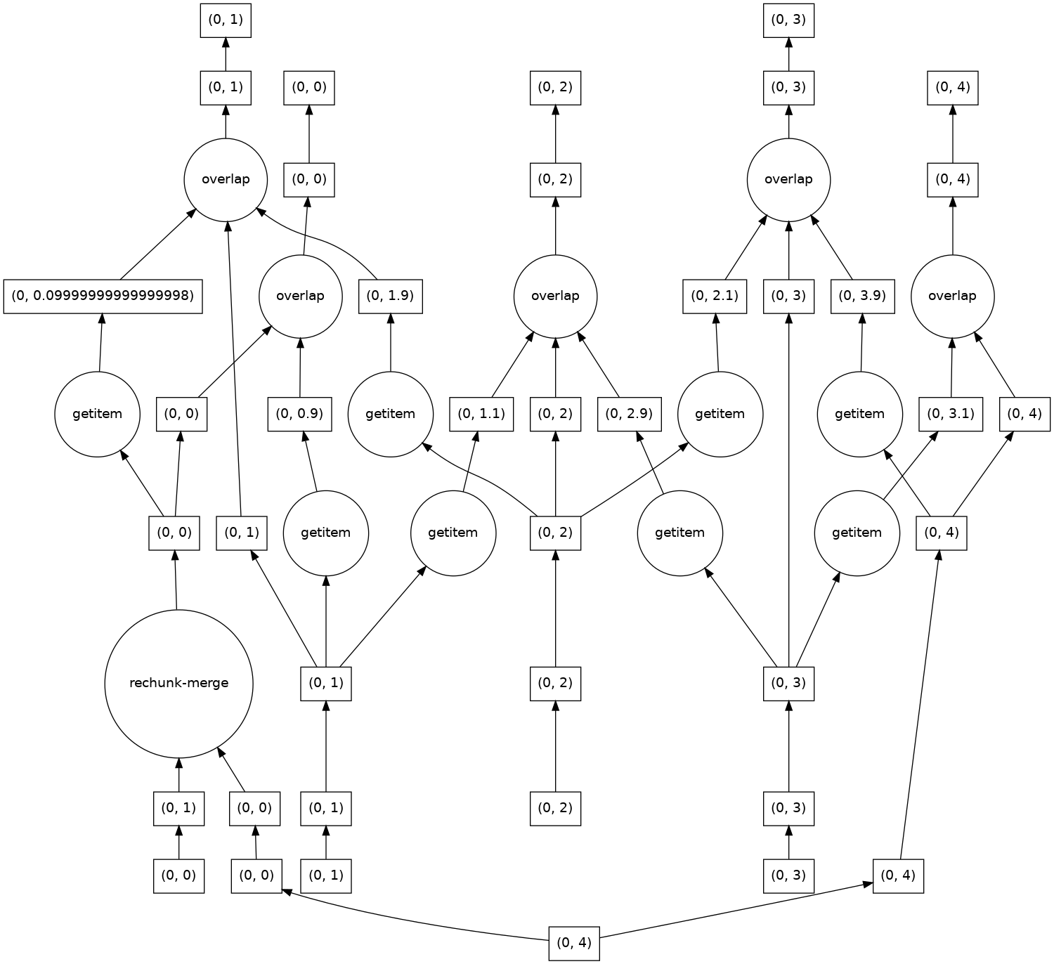
In [49]: result.compute()
Out[49]:
<xarray.DataArray 'x_c' (y: 4, x_g: 9)> Size: 288B
array([[4. , 0.5, 1.5, 2.5, 3.5, 4.5, 5.5, 6.5, 7.5],
       [4. , 0.5, 1.5, 2.5, 3.5, 4.5, 5.5, 6.5, 7.5],
       [4. , 0.5, 1.5, 2.5, 3.5, 4.5, 5.5, 6.5, 7.5],
       [4. , 0.5, 1.5, 2.5, 3.5, 4.5, 5.5, 6.5, 7.5]])
Coordinates:
  * x_g      (x_g) float64 72B 0.5 1.5 2.5 3.5 4.5 5.5 6.5 7.5 8.5
Dimensions without coordinates: y
There is one limitation of this feature: you cannot use map_overlap with grid ufuncs that change length along a core dimension
(e.g. by shifting axis positions from center to outer).
XGCM will raise an error if you try to do this.