Grid Ufunc Examples
This page contains examples of different Grid Ufuncs that you might find useful. They are intended to be more advanced or realistic cases than the simple differencing operations we showed in the introduction to Grid Ufuncs.
As each of these cases is a vector calculus operator, we will demonstrate their use on an example two-dimensional vector field.
Firstly we need a two-dimensional grid, and we use similar coordinate names to the 1D example we used when first introducing Grids.
import numpy as np
import xarray as xr

grid_ds = xr.Dataset(
    coords={
        "x_c": (
            ["x_c"],
            np.arange(1, 20),
            {"axis": "X"},
        ),
        "x_g": (
            ["x_g"],
            np.arange(0.5, 19),
            {"axis": "X", "c_grid_axis_shift": -0.5},
        ),
        "y_c": (
            ["y_c"],
            np.arange(1, 20),
            {"axis": "Y"},
        ),
        "y_g": (
            ["y_g"],
            np.arange(0.5, 19),
            {"axis": "Y", "c_grid_axis_shift": -0.5},
        ),
    }
)
grid_ds
<xarray.Dataset> Size: 608B
Dimensions:  (x_c: 19, x_g: 19, y_c: 19, y_g: 19)
Coordinates:
  * x_c      (x_c) int64 152B 1 2 3 4 5 6 7 8 9 10 11 12 13 14 15 16 17 18 19
  * x_g      (x_g) float64 152B 0.5 1.5 2.5 3.5 4.5 ... 14.5 15.5 16.5 17.5 18.5
  * y_c      (y_c) int64 152B 1 2 3 4 5 6 7 8 9 10 11 12 13 14 15 16 17 18 19
  * y_g      (y_g) float64 152B 0.5 1.5 2.5 3.5 4.5 ... 14.5 15.5 16.5 17.5 18.5
Data variables:
*empty*from xgcm import Grid
grid = Grid(
grid_ds,
coords={
"X": {"center": "x_c", "left": "x_g"},
"Y": {"center": "y_c", "left": "y_g"},
},
boundary="periodic",
autoparse_metadata=False,
)
grid
<xgcm.Grid>
X Axis (periodic, boundary='periodic'):
  * center   x_c --> left
  * left     x_g --> center
Y Axis (periodic, boundary='periodic'):
  * center   y_c --> left
  * left     y_g --> center
Now we need some data.
We will create a 2D vector field, with components U and V.
We will treat these velocities as if they lie on a vector C-grid, so as velocities they will lie at the cell faces.
U = np.sin(grid_ds.x_g * 2 * np.pi / 9.5) * np.cos(grid_ds.y_c * 2 * np.pi / 19)
V = np.cos(grid_ds.x_c * 2 * np.pi / 19) * np.sin(grid_ds.y_g * 2 * np.pi / 19)

ds = xr.Dataset({"V": V, "U": U})
print(ds)
<xarray.Dataset> Size: 6kB
Dimensions:  (x_c: 19, y_g: 19, x_g: 19, y_c: 19)
Coordinates:
  * x_c      (x_c) int64 152B 1 2 3 4 5 6 7 8 9 10 11 12 13 14 15 16 17 18 19
  * y_g      (y_g) float64 152B 0.5 1.5 2.5 3.5 4.5 ... 14.5 15.5 16.5 17.5 18.5
  * x_g      (x_g) float64 152B 0.5 1.5 2.5 3.5 4.5 ... 14.5 15.5 16.5 17.5 18.5
  * y_c      (y_c) int64 152B 1 2 3 4 5 6 7 8 9 10 11 12 13 14 15 16 17 18 19
Data variables:
    V        (x_c, y_g) float64 3kB 0.1557 0.4502 0.6959 ... -0.4759 -0.1646
    U        (x_g, y_c) float64 3kB 0.3071 0.2562 0.1776 ... -0.3071 -0.3247
Interpolation
It would be nice to see what our vector field looks like before we start doing calculus with it,
but the U and V velocities are defined on different points,
so plotting the vectors as arrows originating from a common point would technically be incorrect for our C-grid data.
We can fix this by interpolating the vectors onto co-located points.
colocated = xr.Dataset()
colocated["U"] = grid.interp(U, axis="X", to="center")
colocated["V"] = grid.interp(V, axis="Y", to="center")
colocated
<xarray.Dataset> Size: 6kB
Dimensions:  (x_c: 19, y_c: 19)
Coordinates:
  * x_c      (x_c) int64 152B 1 2 3 4 5 6 7 8 9 10 11 12 13 14 15 16 17 18 19
  * y_c      (y_c) int64 152B 1 2 3 4 5 6 7 8 9 10 11 12 13 14 15 16 17 18 19
Data variables:
    U        (x_c, y_c) float64 3kB 0.5495 0.4584 0.3177 ... 1.388e-16 1.665e-16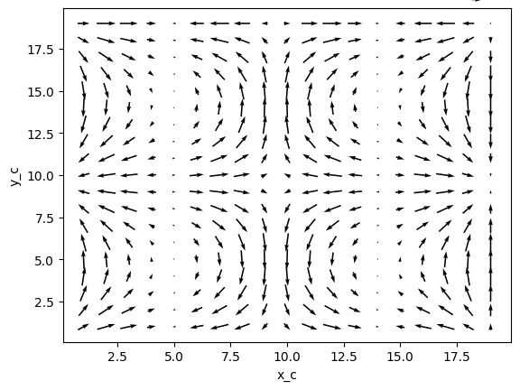
V (x_c, y_c) float64 3kB 0.3029 0.573 0.781 ... -0.3203 8.327e-17We can now show what this co-located vector field looks like
colocated.plot.quiver("x_c", "y_c", u="U", v="V")
/home/docs/checkouts/readthedocs.org/user_builds/xgcm/checkouts/latest/.pixi/envs/docs/lib/python3.13/site-packages/xarray/plot/accessor.py:1160: FutureWarning: Using positional arguments is deprecated for plot methods, use keyword arguments instead.
  return dataset_plot.quiver(self._ds, *args, **kwargs)


<matplotlib.quiver.Quiver at 0x7732e1847cb0>
Divergence
Let's first import the decorator.
from xgcm import as_grid_ufunc
In two dimensions, the divergence operator accepts two vector components and returns one scalar result. A divergence is the sum of multiple partial derivatives, so first let's define a derivative function like this
def diff_forward_1d(a):
    return a[..., 1:] - a[..., :-1]
def diff(arr, axis):
    """First order forward difference along any axis"""
    return np.apply_along_axis(diff_forward_1d, axis, arr)
Each vector component will be differentiated along one axis, and doing so with a first order forward difference would
shift the data's position along that axis.
Therefore our signature should look something like this "(X:left,Y:center),(X:center,Y:left)->(X:center,Y:center)".
We also need to pad the data to replace the elements that will be removed by the diff function, so
our grid ufunc can be defined like this
@as_grid_ufunc(
    "(X:left,Y:center),(X:center,Y:left)->(X:center,Y:center)",
    boundary_width={"X": (0, 1), "Y": (0, 1)},
)
def divergence(u, v):
    u_diff_x = diff(u, axis=-2)
    v_diff_y = diff(v, axis=-1)
    # Need to trim off elements so that the two arrays have same shape
    div = u_diff_x[..., :-1] + v_diff_y[..., :-1, :]
    return div
Here we have treated the components of the (U, V) vector as independent scalars.
Now we can compute the divergence of our example vector field
div = divergence(grid, ds["U"], ds["V"], axis=[("X", "Y"), ("X", "Y")])
We can see the result lies on the expected coordinate positions
div.coords
Coordinates:
  * y_c      (y_c) int64 152B 1 2 3 4 5 6 7 8 9 10 11 12 13 14 15 16 17 18 19
  * x_c      (x_c) int64 152B 1 2 3 4 5 6 7 8 9 10 11 12 13 14 15 16 17 18 19
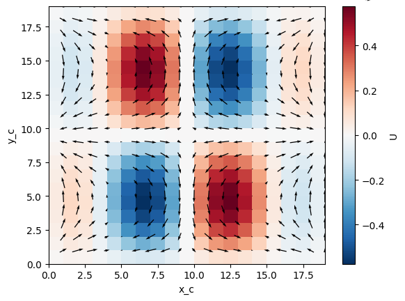
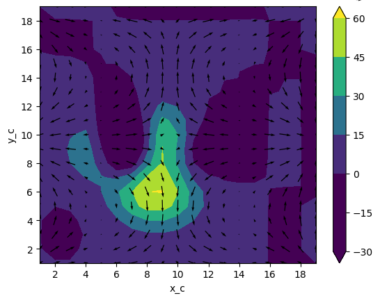
and the resulting divergence looks like it corresponds with the arrows of the vector field above
import matplotlib.pyplot as plt

div.plot(x="x_c", y="y_c")
colocated.plot.quiver("x_c", "y_c", u="U", v="V")
plt.gcf()
/home/docs/checkouts/readthedocs.org/user_builds/xgcm/checkouts/latest/.pixi/envs/docs/lib/python3.13/site-packages/xarray/plot/accessor.py:1160: FutureWarning: Using positional arguments is deprecated for plot methods, use keyword arguments instead.
  return dataset_plot.quiver(self._ds, *args, **kwargs)

Gradient
The gradient is almost like the opposite of divergence in the sense that it accepts one scalar and returns multiple vectors.
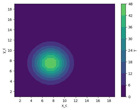
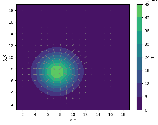
Let's first define a tracer field T, which we imagine will start off localised near the center of the domain.
def gaussian(x_coord, y_coord, x_pos, y_pos, A, w):
    return A * np.exp(-0.5 * ((x_coord - x_pos) ** 2 + (y_coord - y_pos) ** 2) / w**2)
ds["T"] = gaussian(grid_ds.x_c, grid_ds.y_c, x_pos=7.5, y_pos=7.5, A=50, w=2)
ds["T"].plot.contourf(x="x_c", vmax=60)
<matplotlib.contour.QuadContourSet at 0x7732e16a9be0>
Computing the first-order gradient will again move the data onto different grid positions, so the signature for a gradient ufunc will need to reflect this and our definition is similar to the derivative case.
def gradient(a):
    a_diff_x = diff(a, axis=-2)
    a_diff_y = diff(a, axis=-1)
    # Need to trim off elements so that the two arrays have same shape
    return a_diff_x[..., :-1], a_diff_y[..., :-1, :]
Now we can compute the gradient of our example scalar field
ds["grad_T_x"], ds["grad_T_y"] = grid.apply_as_grid_ufunc(
    gradient,
    ds["T"],
    axis=[("X", "Y")],
    signature="(X:center,Y:center)->(X:left,Y:center),(X:center,Y:left)",
    boundary_width={"X": (1, 0), "Y": (1, 0)},
)
Note
Notice we used the apply_as_grid_ufunc syntax here instead of the as_grid_ufunc decorator.
The result is the same.
Again in order to plot this as a vector field we should first interpolate it
colocated["grad_T_x"] = grid.interp(ds["grad_T_x"], axis="X", to="center")
colocated["grad_T_y"] = grid.interp(ds["grad_T_y"], axis="Y", to="center")
colocated
<xarray.Dataset> Size: 12kB
Dimensions:   (x_c: 19, y_c: 19)
Coordinates:
  * x_c       (x_c) int64 152B 1 2 3 4 5 6 7 8 9 10 11 12 13 14 15 16 17 18 19
  * y_c       (y_c) int64 152B 1 2 3 4 5 6 7 8 9 10 11 12 13 14 15 16 17 18 19
Data variables:
    U         (x_c, y_c) float64 3kB 0.5495 0.4584 ... 1.388e-16 1.665e-16
    V         (x_c, y_c) float64 3kB 0.3029 0.573 0.781 ... -0.3203 8.327e-17
    grad_T_x  (x_c, y_c) float64 3kB 3.77e-08 0.002898 ... 1.603e-06 1.316e-07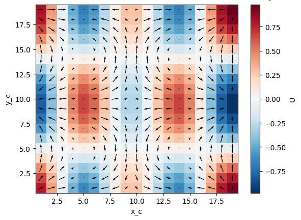
grad_T_y (x_c, y_c) float64 3kB 3.77e-08 1.232e-07 ... -3.245e-10 1.316e-07Now we can plot the gradient of the tracer field as a vector field
ds["T"].plot.contourf(x="x_c", vmax=60)
colocated.plot.quiver("x_c", "y_c", u="grad_T_x", v="grad_T_y", color="0.5", scale=200)
plt.gcf()

Advection
We can also do "mixed" operations that involve both vectors and scalars, such as calculating the advective flux of a scalar tracer field due to a vector flow field.
Now we can define a simple flux operator (which internally calls our previous gradient function)
def interp_forward_1d(a):
    return (a[..., :-1] + a[..., 1:]) / 2.0
def interp_forward(arr, axis):
    """First order forward interpolation along any axis"""
    return np.apply_along_axis(interp_forward_1d, axis, arr)
@as_grid_ufunc(
    "(X:left,Y:center),(X:center,Y:left),(X:center,Y:center)->(X:left,Y:center),(X:center,Y:left)",
    boundary_width={"X": (1, 0), "Y": (1, 0)},
)
def flux(u, v, T):
    """First order flux"""
    T_at_U_position = interp_forward(T, axis=-2)
    T_at_V_position = interp_forward(T, axis=-1)
    T_flux_x = u[..., :-1, :-1] * T_at_U_position[..., :-1]
    T_flux_y = v[..., :-1, :-1] * T_at_V_position[..., :-1, :]
    return T_flux_x, T_flux_y
We can use this operator in conjunction with our divergence operator in order to build an advection operator, with which we can solve the basic continuity equation
def advect(T, U, V, delta_t):
    """Simple solution to the continuity equation for a single timestep of length delta_t."""
    T_flux_x, T_flux_y = flux(grid, U, V, T, axis=[("X", "Y")] * 3)
    advected_T = T - delta_t * divergence(
        grid, T_flux_x, T_flux_y, axis=[("X", "Y")] * 2
    )
    return advected_T
Evaluating this function updates our tracer to what the tracer field might look like one (arbitrary-length) timestep later:
new_T = advect(ds["T"], ds["U"], ds["V"], delta_t=3)

new_T.plot.contourf(x="x_c", vmin=0, vmax=60)
colocated.plot.quiver("x_c", "y_c", u="U", v="V")
plt.gcf()

Vorticity
We can compute vector fields from vector fields too, such as vorticity.
@as_grid_ufunc(
    "(X:left,Y:center),(X:center,Y:left)->(X:left,Y:left)",
    boundary_width={"X": (1, 0), "Y": (1, 0)},
)
def vorticity(u, v):
    v_diff_x = diff(v, axis=-2)
    u_diff_y = diff(u, axis=-1)
    return v_diff_x[..., 1:] - u_diff_y[..., 1:, :]
vort = vorticity(grid, ds["U"], ds["V"], axis=[("X", "Y"), ("X", "Y")])
vort.plot(x="x_g", y="y_g")
colocated.plot.quiver("x_c", "y_c", u="U", v="V")
plt.gcf()