Grid Topology¶

Warning

The features described in this page should be considered experimental. The API is subject to change. Please report any unexpected behavior or unpleasant experiences on the github issues page

Faces and Connections¶

Simple grids, as described on the Grids page, consist of a single logically rectangular domain. Many modern GCMs use more complex grid topologies, consisting of multiple logically rectangular grids connected at their edges. xgcm is capable of understanding the connections between these grid faces and exchanging data between them appropriately.

Cubed Sphere Grid

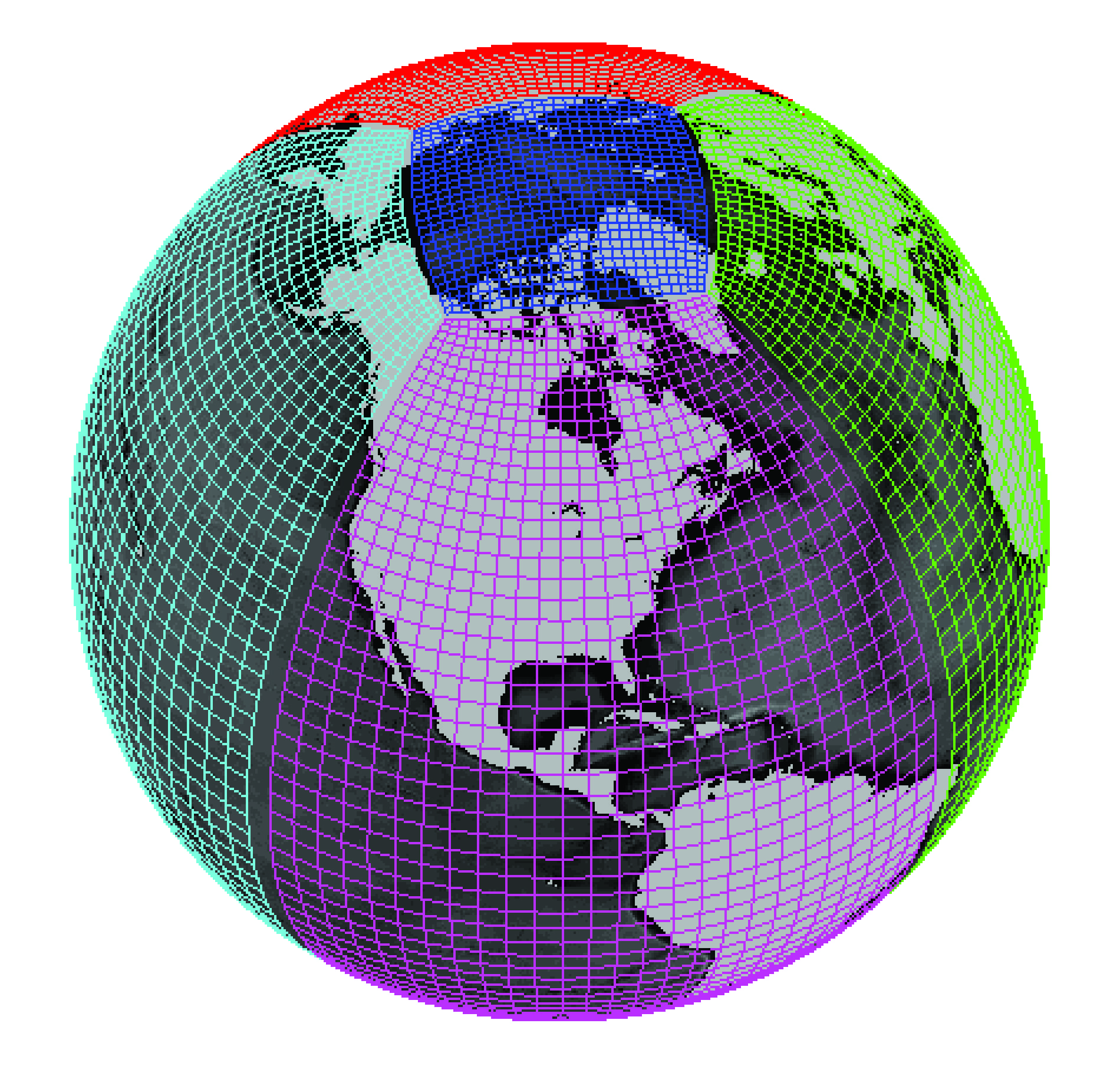
Example of a lat-lon-cap grid from the MIT General Circulation Model. Image credit Gael Forget. More information about the simulation and grid available at https://doi.org/10.5194/gmd-8-3071-2015.

In order to construct such a complex grid topology, we need a way to tell xgcm about the connections between faces. This is accomplished via the face_connections keyword argument to the Grid constructor. Below we illustrate how this works with a series of increasingly complex examples. If you just want to get the detailed specifications for face_connections, jump down to Face Connections Spec.

Examples¶

Two Connected Faces¶

The simplest possible scenario is two faces connected at one side. Consider the following dataset

import numpy as np
import xarray as xr

N = 25
ds = xr.Dataset(
    {"data_c": (["face", "y", "x"], np.random.rand(2, N, N))},
    coords={
        "x": (("x",), np.arange(N), {"axis": "X"}),
        "xl": (
            ("xl"),
            np.arange(N) - 0.5,
            {"axis": "X", "c_grid_axis_shift": -0.5},
        ),
        "y": (("y",), np.arange(N), {"axis": "Y"}),
        "yl": (
            ("yl"),
            np.arange(N) - 0.5,
            {"axis": "Y", "c_grid_axis_shift": -0.5},
        ),
        "face": (("face",), [0, 1]),
    },
)
print(ds)

<xarray.Dataset> Size: 11kB
Dimensions:  (face: 2, y: 25, x: 25, xl: 25, yl: 25)
Coordinates:
  * face     (face) int64 16B 0 1
  * y        (y) int64 200B 0 1 2 3 4 5 6 7 8 9 ... 16 17 18 19 20 21 22 23 24
  * x        (x) int64 200B 0 1 2 3 4 5 6 7 8 9 ... 16 17 18 19 20 21 22 23 24
  * xl       (xl) float64 200B -0.5 0.5 1.5 2.5 3.5 ... 19.5 20.5 21.5 22.5 23.5
  * yl       (yl) float64 200B -0.5 0.5 1.5 2.5 3.5 ... 19.5 20.5 21.5 22.5 23.5
Data variables:
    data_c   (face, y, x) float64 10kB 0.8017 0.5746 0.352 ... 0.8597 0.4602

The dataset has two spatial axes (X and Y), plus an additional dimension face of length 2. Let's imagine the two faces are joined in the following way:

two connected faces

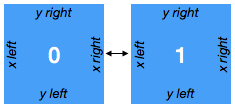
We can construct a grid that understands this connection in the following way:

import xgcm

face_connections = {
    "face": {0: {"X": (None, (1, "X", False))}, 1: {"X": ((0, "X", False), None)}}
}
grid = xgcm.Grid(ds, face_connections=face_connections)
grid

<xgcm.Grid>
X Axis (not periodic, padding=None):
  * center   x --> left
  * left     xl --> center
Y Axis (not periodic, padding=None):
  * center   y --> left
  * left     yl --> center

The face_connections dictionary tells xgcm that face is the name of the dimension that contains the different faces. (It might have been called tile or facet or something else similar.) This dictionary say that face number 0 is connected along the X axis to nothing on the left and to face number 1 on the right. A complementary connection exists from face number 1. These connections are checked for consistency.

We can now use Grid.interp and Grid.diff to correctly interpolate and difference across the connected faces.

Two Faces with Rotated Axes¶

face_connections = {
    "face": {0: {"X": (None, (1, "Y", False))}, 1: {"Y": ((0, "X", False), None)}}
}
grid = xgcm.Grid(ds, face_connections=face_connections)
grid

<xgcm.Grid>
X Axis (not periodic, padding=None):
  * center   x --> left
  * left     xl --> center
Y Axis (not periodic, padding=None):
  * center   y --> left
  * left     yl --> center

Cubed Sphere¶

A more realistic and complicated example is a cubed sphere. One possible topology for a cubed sphere grid is shown in the figure below:

cubed sphere face connections

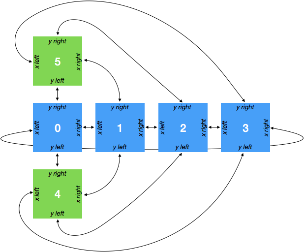
This geometry has six faces. We can generate an xarray Dataset that has two spatial dimensions and a face dimension as follows:

ds = xr.Dataset(
    {"data_c": (["face", "y", "x"], np.random.rand(6, N, N))},
    coords={
        "x": (("x",), np.arange(N), {"axis": "X"}),
        "xl": (
            ("xl"),
            np.arange(N) - 0.5,
            {"axis": "X", "c_grid_axis_shift": -0.5},
        ),
        "y": (("y",), np.arange(N), {"axis": "Y"}),
        "yl": (
            ("yl"),
            np.arange(N) - 0.5,
            {"axis": "Y", "c_grid_axis_shift": -0.5},
        ),
        "face": (("face",), np.arange(6)),
    },
)
print(ds)

<xarray.Dataset> Size: 31kB
Dimensions:  (face: 6, y: 25, x: 25, xl: 25, yl: 25)
Coordinates:
  * face     (face) int64 48B 0 1 2 3 4 5
  * y        (y) int64 200B 0 1 2 3 4 5 6 7 8 9 ... 16 17 18 19 20 21 22 23 24
  * x        (x) int64 200B 0 1 2 3 4 5 6 7 8 9 ... 16 17 18 19 20 21 22 23 24
  * xl       (xl) float64 200B -0.5 0.5 1.5 2.5 3.5 ... 19.5 20.5 21.5 22.5 23.5
  * yl       (yl) float64 200B -0.5 0.5 1.5 2.5 3.5 ... 19.5 20.5 21.5 22.5 23.5
Data variables:
    data_c   (face, y, x) float64 30kB 0.9369 0.6316 0.8481 ... 0.8436 0.4314

We specify the face connections and create the Grid object as follows:

face_connections = {
    "face": {
        0: {
            "X": ((3, "X", False), (1, "X", False)),
            "Y": ((4, "Y", False), (5, "Y", False)),
        },
        1: {
            "X": ((0, "X", False), (2, "X", False)),
            "Y": ((4, "X", False), (5, "X", True)),
        },
        2: {
            "X": ((1, "X", False), (3, "X", False)),
            "Y": ((4, "Y", True), (5, "Y", True)),
        },
        3: {
            "X": ((2, "X", False), (0, "X", False)),
            "Y": ((4, "X", True), (5, "X", False)),
        },
        4: {
            "X": ((3, "Y", True), (1, "Y", False)),
            "Y": ((2, "Y", True), (0, "Y", False)),
        },
        5: {
            "X": ((3, "Y", False), (1, "Y", True)),
            "Y": ((0, "Y", False), (2, "Y", True)),
        },
    }
}
grid = xgcm.Grid(ds, face_connections=face_connections)
grid

<xgcm.Grid>
X Axis (not periodic, padding=None):
  * center   x --> left
  * left     xl --> center
Y Axis (not periodic, padding=None):
  * center   y --> left
  * left     yl --> center

For a real-world example of how to use face connections, check out the MITgcm ECCOv4 example.

Face Connections Spec¶

Because of the diversity of different model grid topologies, xgcm tries to avoid making assumptions about the nature of the connectivity between faces. It is up to the user to specify this connectivity via the face_connections dictionary. The face_connections dictionary has the following general stucture

{'<FACE DIMENSION NAME>':
    {<FACE DIMENSION VALUE>:
         {'<AXIS NAME>': (<LEFT CONNECTION>, <RIGHT CONNECTION>),
          ...}
    ...
}

<LEFT CONNECTION>> and <RIGHT CONNECTION> are either None (for no connection) or a three element tuple with the following contents

(<FACE DIMENSION VALUE>, `<AXIS NAME>`, <REVERSE CONNECTION>)

<FACE DIMENSION VALUE> tells which face this face is connected to. <AXIS NAME> tells which axis on that face is connected to this one. <REVERSE CONNECTION> is a boolean specifying whether the connection is "reversed". A normal (non reversed) connection connects the right edge of one face to the left edge of another face. A reversed connection connects left to left, or right to right.

Note

We may consider adding standard face_connections dictionaries for common models (e.g. MITgcm, GEOS, etc.) as a convenience within xgcm. If you would like to pursue this, please open a github issue.

The Bipolar North Fold (Tripolar Grids)¶

Experimental

The north fold is experimental. Its API (how the fold pivot and seam are declared) and its numerical behavior may change in future releases, and it has not yet been validated across the full range of grid configurations and models. Constructing a Grid with a fold boundary emits a UserWarning to this effect. Please check results carefully and report any issues on the issue tracker.

Many global ocean models (e.g. MOM6/OM4, NEMO/ORCA, MOM5, Oceananigans) avoid the coordinate singularity at the geographic North Pole by displacing it onto land and pairing it with a second displaced pole. Such grids are called tripolar: they carry three singularities — the ordinary South Pole plus the two Arctic poles. Logically the grid is still a single rectangular tile, but its northern edge folds onto itself along the bipolar seam, the line joining the two northern poles; the top row is welded to a mirror-image of itself running the other way.

So the two words describe different things: the grid is tripolar (three poles), while the fold — this boundary condition — is bipolar (its seam connects the two northern poles). xgcm calls the feature a north fold.

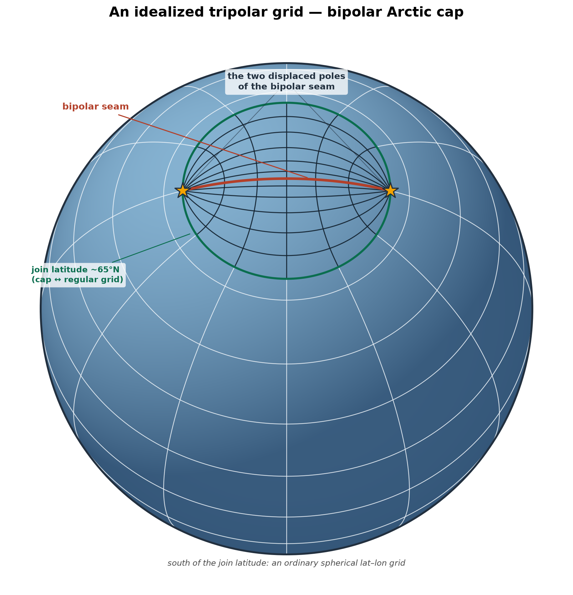
An idealized tripolar grid on the globe

An idealized tripolar grid. South of a chosen join latitude (here ~65°N) the mesh is an ordinary spherical lat–lon grid; north of it a bipolar Arctic cap carries the grid's two displaced northern poles (stars), joined by the bipolar seam that folds the northern edge onto itself and passes through the geographic North Pole. Together with the ordinary South Pole, those two Arctic poles are the three singularities that make the grid tripolar. The cap is a conformal bipolar projection (Murray 1996) whose grid lines join the regular grid continuously at the join latitude; generated by scripts/make_tripolar_grid.py.

Because the fold lives on the upper edge of one tile — not between separate faces — it is not a face connection. Instead it is requested as a per-axis padding value on the meridional (fold) axis, with the zonal (seam) axis marked periodic:

import numpy as np
import xarray as xr
import xgcm

N = 8
ds = xr.Dataset(
    coords={
        "x_c": ("x_c", np.arange(N)),
        "x_g": ("x_g", np.arange(N) - 0.5),
        "y_c": ("y_c", np.arange(N)),
        "y_g": ("y_g", np.arange(N) - 0.5),
    },
)
ds["sst"] = (("y_c", "x_c"), np.cos(2 * np.pi * np.arange(N) / N) + np.zeros((N, 1)))

grid = xgcm.Grid(
    ds,
    coords={
        "X": {"center": "x_c", "left": "x_g"},
        "Y": {"center": "y_c", "left": "y_g"},
    },
    padding={"X": "periodic", "Y": {"fold": "corner"}},
    autoparse_metadata=False,
)
grid

/home/docs/checkouts/readthedocs.org/user_builds/xgcm/checkouts/latest/xgcm/grid.py:463: UserWarning: The north-fold (tripolar) boundary condition is experimental. Its API and numerical behavior may change in future releases, and it has not yet been validated across the full range of grid configurations. Please review results carefully and report any issues at https://github.com/xgcm/xgcm/issues.
  warnings.warn(





<xgcm.Grid>
X Axis (periodic, padding='periodic'):
  * center   x_c --> left
  * left     x_g --> center
Y Axis (not periodic, padding={'fold': 'corner', 'south': 'fill'}):
  * center   y_c --> left
  * left     y_g --> center

The seam axis is inferred as the axis you explicitly mark "periodic". On a 3-D grid you therefore only need to declare the zonal seam ("X") and the fold ("Y"); a vertical axis can be left unspecified and will not be mistaken for the seam. The inference is only ambiguous if you explicitly mark more than one non-fold axis periodic.

With the fold in place, interp, diff, derivative, and the rest of the grid operators stitch correctly across the top edge instead of falling back to an ordinary boundary. To see what the fold actually does, label each cell of the northern row by its column index and pad a single halo row across the seam — the halo comes back as the interior row mirrored about the pole:

from xgcm.padding import pad

cols = xr.DataArray(np.broadcast_to(np.arange(N), (N, N)), dims=("y_c", "x_c"))
halo = pad(cols, grid, padding_width={"Y": (0, 1)}).isel(y_c=-1)

print("interior north row (cells labelled by column):", cols.isel(y_c=-1).values)
print("folded halo row    (mirrored about the pole) :", halo.values)

interior north row (cells labelled by column): [0 1 2 3 4 5 6 7]
folded halo row    (mirrored about the pole) : [7 6 5 4 3 2 1 0]

Every Grid operator that reaches across the northern edge — grid.diff(ds.sst, "Y"), grid.interp, grid.derivative, … — pads this halo automatically.

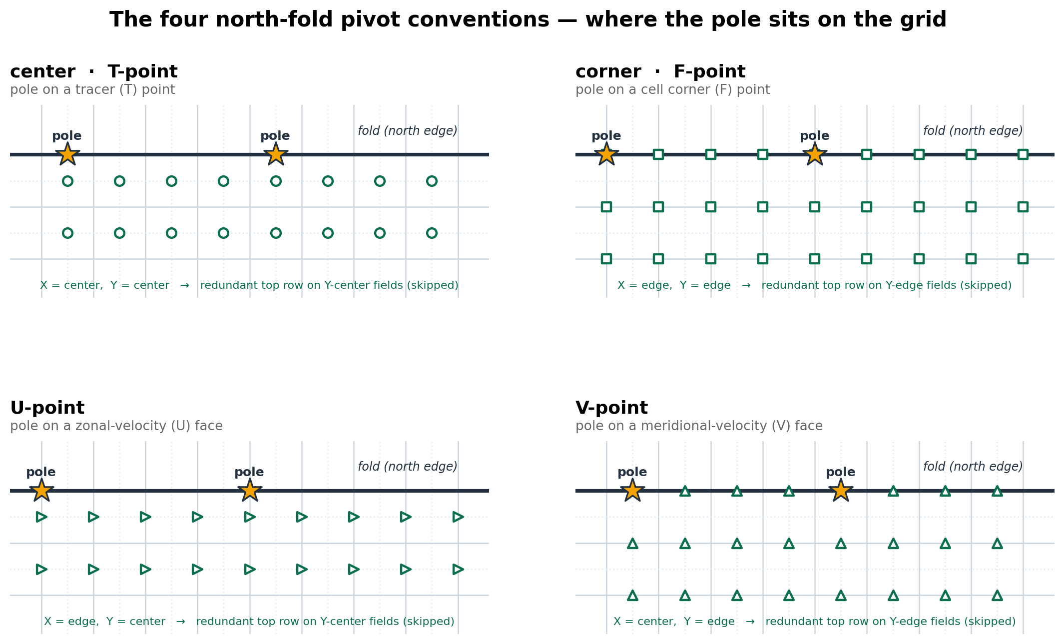
The four pivot conventions¶

The value of "fold" names the pivot: the staggered grid position that the fold's fixed point (the pole) sits on. A C-grid stores variables at four kinds of position — tracer centers (T), cell corners (F), and the two velocity faces (U, V) — so there are four conventions, and the seam reflects each field about the pole that matches its position:

The four north-fold pivot conventions

`fold` value	Aliases	Pole position (X, Y)	Pole sits on
`"center"`	`"t"`	center, center	a tracer (T) point
`"corner"`	`"f"`	edge, edge	a cell corner (F) point
`"u"`		edge, center	a zonal-velocity (U) face
`"v"`		center, edge	a meridional-velocity (V) face

The seam is bipolar: a periodic reflection has two fixed points, half a domain apart (the stars above). Whether the pole sits on a cell edge or a cell center in X sets their zonal location; whether it sits on an edge or center in Y sets, for each field separately, whether that field's topmost row lies exactly on the fold line — a redundant row, which xgcm skips — or half a cell below it. A field's top row is on the line precisely when the field's own Y position (center or edge) matches the pivot's; so a pivot whose pole is Y-centered (center/u) still produces a redundant top row for its center-positioned fields, not only the Y-edge pivots (corner/v).

These four exhaust the possibilities — the pivot depends only on whether each axis lands on a cell center or a cell edge, and a center/edge pair on each of two axes is four cases. If you would rather name the positions directly than recall the T/F/U/V vocabulary, pass an explicit {axis: position} mapping using your grid's own axis names; it resolves to the same four. For example {"fold": {"X": "center", "Y": "left"}} is just another way to write "v" (any non-center Y position — left, right, inner, outer — counts as an edge).

How the halo is filled¶

To evaluate an operator across the top edge, xgcm pads a northern halo by reflecting the interior about the nearest pole. A scalar (tracer, layer thickness, …) is mirrored as-is; a vector component (a velocity, a flux) is mirrored and sign-flipped, because folding the grid rotates the local axes by 180°:

How the north fold fills the halo

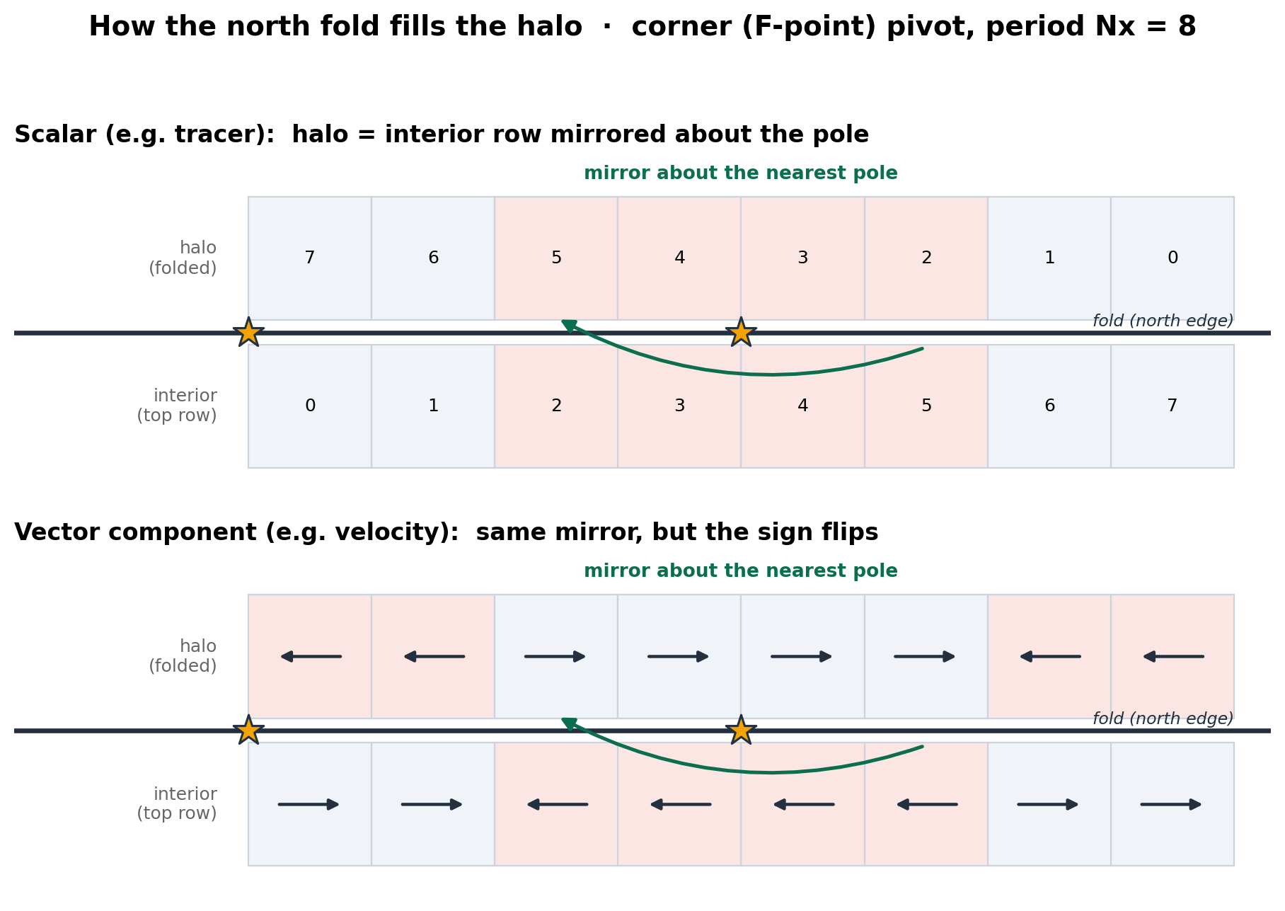
To fold a field as a vector (so its components flip sign), pass it wrapped as a single-key dict keyed by its axis, e.g. {"X": ds.u} — that is what flags it as a vector rather than a scalar. Unlike a 90° rotated face connection, the 180° fold needs no partner component (each component simply reverses sign), so other_component is optional here. Folding the same u data as a scalar versus as a vector shows the difference — the vector halo is the scalar halo with the sign reversed:

ds["u"] = (("y_c", "x_g"), np.broadcast_to(np.arange(1, N + 1), (N, N)).astype(float))
ds["v"] = (("y_g", "x_c"), np.zeros((N, N)))  # U-point / V-point components

scalar = pad(ds.u, grid, padding_width={"Y": (0, 1)}).isel(y_c=-1)
vector = pad(
    {"X": ds.u}, grid, padding_width={"Y": (0, 1)}, other_component={"Y": ds.v}
).isel(y_c=-1)

print("u folded as a scalar (mirror)            :", scalar.values)
print("u folded as a vector (mirror + sign flip):", vector.values)

u folded as a scalar (mirror)            : [1. 8. 7. 6. 5. 4. 3. 2.]
u folded as a vector (mirror + sign flip): [-1. -8. -7. -6. -5. -4. -3. -2.]

The same applies to the high-level operators: grid.diff({"X": ds.u}, "Y", other_component={"Y": ds.v}) differences the u component across the fold with the sign handled for you.

The fold is applied purely in the padding layer as an indexed gather, so it stays lazy and works with multi-chunk dask arrays. For a worked example on real model output from three different codes — including interp (surface speed) and diff (horizontal divergence) diagnostics that stay continuous across the seam — see the Tripolar fold example.

Note

Only the north edge folds; the south edge of the fold axis uses an ordinary boundary — a per-call padding passed to the operator if given, otherwise the construction-time "south" mode (default fill), set via the "south" key, e.g. {"fold": "corner", "south": "extend"}.