MITgcm Example#
xgcm is developed in close coordination with the xmitgcm package. The metadata in datasets constructed by xmitgcm should always be compatible with xgcm’s expectations. xmitgcm is necessary for reading MITgcm’s binary MDS file format. However, for this example, the MDS files have already been converted and saved as netCDF.
Below are some example of how to make calculations on mitgcm-style datasets using xgcm.
First we import xarray and xgcm:
[1]:
import xarray as xr
import numpy as np
import xgcm
from matplotlib import pyplot as plt
%matplotlib inline
plt.rcParams['figure.figsize'] = (10,6)
Now we open the example dataset which is stored in a zenodo archive.
[3]:
# download the data
import urllib.request
import shutil

url = 'https://zenodo.org/record/4421428/files/'
file_name = 'mitgcm_example_dataset_v2.nc'
with urllib.request.urlopen(url + file_name) as response, open(file_name, 'wb') as out_file:
    shutil.copyfileobj(response, out_file)

# open the data
ds = xr.open_dataset(file_name)
ds
[3]:
<xarray.Dataset>
Dimensions:  (XC: 90, XG: 90, YC: 40, YG: 40, Z: 15, Zl: 15, time: 1)
Coordinates:
  * time     (time) timedelta64[ns] 11:00:00
    maskC    (Z, YC, XC) bool False False False False ... False False False
    dyC      (YG, XC) float32 4.447e+05 4.447e+05 ... 4.447e+05 4.447e+05
    hFacC    (Z, YC, XC) float32 0.0 0.0 0.0 0.0 0.0 0.0 ... 0.0 0.0 0.0 0.0 0.0
    rA       (YC, XC) float32 4.111e+10 4.111e+10 ... 4.111e+10 4.111e+10
    hFacS    (Z, YG, XC) float32 0.0 0.0 0.0 0.0 0.0 0.0 ... 0.0 0.0 0.0 0.0 0.0
    Depth    (YC, XC) float32 0.0 0.0 0.0 0.0 ... 187.5 1.917e+03 2.995e+03
  * YG       (YG) float32 -80.0 -76.0 -72.0 -68.0 -64.0 ... 64.0 68.0 72.0 76.0
  * Z        (Z) float32 -25.0 -85.0 -170.0 ... -3.575e+03 -4.19e+03 -4.855e+03
    PHrefC   (Z) float32 245.2 833.8 1.668e+03 ... 3.507e+04 4.11e+04 4.763e+04
    dyG      (YC, XG) float32 4.447e+05 4.447e+05 ... 4.447e+05 4.447e+05
    rAw      (YC, XG) float32 4.111e+10 4.111e+10 ... 4.111e+10 4.111e+10
    drF      (Z) float32 50.0 70.0 100.0 140.0 190.0 ... 540.0 590.0 640.0 690.0
  * YC       (YC) float32 -78.0 -74.0 -70.0 -66.0 -62.0 ... 66.0 70.0 74.0 78.0
    dxG      (YG, XC) float32 7.722e+04 7.722e+04 ... 1.076e+05 1.076e+05
  * XG       (XG) float32 0.0 4.0 8.0 12.0 16.0 ... 344.0 348.0 352.0 356.0
    iter     (time) int64 39600
    maskW    (Z, YC, XG) bool False False False False ... False False False
  * Zl       (Zl) float32 0.0 -50.0 -120.0 ... -3.28e+03 -3.87e+03 -4.51e+03
    rAs      (YG, XC) float32 3.433e+10 3.433e+10 ... 4.783e+10 4.783e+10
    rAz      (YG, XG) float32 3.433e+10 3.433e+10 ... 4.783e+10 4.783e+10
    maskS    (Z, YG, XC) bool False False False False ... False False False
    dxC      (YC, XG) float32 9.246e+04 9.246e+04 ... 9.246e+04 9.246e+04
    hFacW    (Z, YC, XG) float32 0.0 0.0 0.0 0.0 0.0 0.0 ... 0.0 0.0 0.0 0.0 0.0
  * XC       (XC) float32 2.0 6.0 10.0 14.0 18.0 ... 346.0 350.0 354.0 358.0
Data variables:
    UVEL     (time, Z, YC, XG) float32 0.0 0.0 0.0 0.0 0.0 ... 0.0 0.0 0.0 0.0
    VVEL     (time, Z, YG, XC) float32 0.0 0.0 0.0 0.0 0.0 ... 0.0 0.0 0.0 0.0
    WVEL     (time, Zl, YC, XC) float32 0.0 0.0 0.0 0.0 0.0 ... 0.0 0.0 0.0 0.0
    SALT     (time, Z, YC, XC) float32 0.0 0.0 0.0 0.0 0.0 ... 0.0 0.0 0.0 0.0
    THETA    (time, Z, YC, XC) float32 0.0 0.0 0.0 0.0 0.0 ... 0.0 0.0 0.0 0.0
    PH       (time, Z, YC, XC) float32 -8.3 -8.3 -8.3 ... -470.8 -202.8
    Eta      (time, YC, XC) float32 0.0 0.0 0.0 0.0 ... -0.6293 -0.6234 -0.649
Attributes:
    Conventions:  CF-1.6
    title:        netCDF wrapper of MITgcm MDS binary data
    source:       MITgcm
history: Created by calling `open_mdsdataset(extra_metadata=None, ll...- XC: 90
- XG: 90
- YC: 40
- YG: 40
- Z: 15
- Zl: 15
- time: 1
- time(time)timedelta64[ns]11:00:00
- standard_name :
- time
- long_name :
- Time
- axis :
- T
- calendar :
- gregorian
array([39600000000000], dtype='timedelta64[ns]')
- maskC(Z, YC, XC)bool...
- standard_name :
- sea_binary_mask_at_t_location
- long_name :
- mask denoting wet point at center
array([[[False, False, ..., False, False], [False, False, ..., False, False], ..., [ True, True, ..., True, True], [ True, True, ..., True, True]], [[False, False, ..., False, False], [False, False, ..., False, False], ..., [ True, True, ..., True, True], [ True, True, ..., True, True]], ..., [[False, False, ..., False, False], [False, False, ..., False, False], ..., [False, False, ..., False, False], [False, False, ..., False, False]], [[False, False, ..., False, False], [False, False, ..., False, False], ..., [False, False, ..., False, False], [False, False, ..., False, False]]]) - dyC(YG, XC)float32...
- standard_name :
- cell_y_size_at_v_location
- long_name :
- cell y size
- units :
- m
- coordinate :
- YG XC
array([[444709.9, 444709.9, 444709.9, ..., 444709.9, 444709.9, 444709.9], [444709.9, 444709.9, 444709.9, ..., 444709.9, 444709.9, 444709.9], [444709.9, 444709.9, 444709.9, ..., 444709.9, 444709.9, 444709.9], ..., [444709.9, 444709.9, 444709.9, ..., 444709.9, 444709.9, 444709.9], [444709.9, 444709.9, 444709.9, ..., 444709.9, 444709.9, 444709.9], [444709.9, 444709.9, 444709.9, ..., 444709.9, 444709.9, 444709.9]], dtype=float32) - hFacC(Z, YC, XC)float32...
- standard_name :
- cell_vertical_fraction
- long_name :
- vertical fraction of open cell
array([[[0., 0., ..., 0., 0.], [0., 0., ..., 0., 0.], ..., [1., 1., ..., 1., 1.], [1., 1., ..., 1., 1.]], [[0., 0., ..., 0., 0.], [0., 0., ..., 0., 0.], ..., [1., 1., ..., 1., 1.], [1., 1., ..., 1., 1.]], ..., [[0., 0., ..., 0., 0.], [0., 0., ..., 0., 0.], ..., [0., 0., ..., 0., 0.], [0., 0., ..., 0., 0.]], [[0., 0., ..., 0., 0.], [0., 0., ..., 0., 0.], ..., [0., 0., ..., 0., 0.], [0., 0., ..., 0., 0.]]], dtype=float32) - rA(YC, XC)float32...
- standard_name :
- cell_area
- long_name :
- cell area
- units :
- m2
- coordinate :
- YC XC
array([[4.110970e+10, 4.110970e+10, 4.110970e+10, ..., 4.110970e+10, 4.110970e+10, 4.110970e+10], [5.450087e+10, 5.450087e+10, 5.450087e+10, ..., 5.450087e+10, 5.450087e+10, 5.450087e+10], [6.762652e+10, 6.762652e+10, 6.762652e+10, ..., 6.762652e+10, 6.762652e+10, 6.762652e+10], ..., [6.762652e+10, 6.762652e+10, 6.762652e+10, ..., 6.762652e+10, 6.762652e+10, 6.762652e+10], [5.450087e+10, 5.450087e+10, 5.450087e+10, ..., 5.450087e+10, 5.450087e+10, 5.450087e+10], [4.110970e+10, 4.110970e+10, 4.110970e+10, ..., 4.110970e+10, 4.110970e+10, 4.110970e+10]], dtype=float32) - hFacS(Z, YG, XC)float32...
- standard_name :
- cell_vertical_fraction_at_v_location
- long_name :
- vertical fraction of open cell
array([[[0., 0., ..., 0., 0.], [0., 0., ..., 0., 0.], ..., [1., 1., ..., 1., 1.], [1., 1., ..., 1., 1.]], [[0., 0., ..., 0., 0.], [0., 0., ..., 0., 0.], ..., [1., 1., ..., 1., 1.], [1., 1., ..., 1., 1.]], ..., [[0., 0., ..., 0., 0.], [0., 0., ..., 0., 0.], ..., [0., 0., ..., 0., 0.], [0., 0., ..., 0., 0.]], [[0., 0., ..., 0., 0.], [0., 0., ..., 0., 0.], ..., [0., 0., ..., 0., 0.], [0., 0., ..., 0., 0.]]], dtype=float32) - Depth(YC, XC)float32...
- standard_name :
- ocean_depth
- long_name :
- ocean depth
- units :
- m
- coordinate :
- XC YC
array([[ 0. , 0. , 0. , ..., 0. , 0. , 0. ], [ 0. , 0. , 0. , ..., 0. , 0. , 0. ], [3740. , 3671.5, 1732.5, ..., 3821. , 4047.5, 4047.5], ..., [2144. , 2214.5, 2414. , ..., 1586.5, 2703. , 2048.5], [2995. , 2414. , 2414. , ..., 1183. , 1569.5, 2995. ], [2995. , 2354.5, 2087. , ..., 187.5, 1917. , 2995. ]], dtype=float32) - YG(YG)float32-80.0 -76.0 -72.0 ... 72.0 76.0
- standard_name :
- latitude_at_f_location
- long_name :
- latitude
- units :
- degrees_north
- axis :
- Y
- c_grid_axis_shift :
- -0.5
array([-80., -76., -72., -68., -64., -60., -56., -52., -48., -44., -40., -36., -32., -28., -24., -20., -16., -12., -8., -4., 0., 4., 8., 12., 16., 20., 24., 28., 32., 36., 40., 44., 48., 52., 56., 60., 64., 68., 72., 76.], dtype=float32) - Z(Z)float32-25.0 -85.0 ... -4.855e+03
- standard_name :
- depth
- long_name :
- vertical coordinate of cell center
- units :
- m
- positive :
- down
- axis :
- Z
array([ -25., -85., -170., -290., -455., -670., -935., -1250., -1615., -2030., -2495., -3010., -3575., -4190., -4855.], dtype=float32) - PHrefC(Z)float32...
- standard_name :
- cell_reference_pressure
- long_name :
- Reference Hydrostatic Pressure
- units :
- m2 s-2
array([ 245.25, 833.85, 1667.7 , 2844.9 , 4463.55, 6572.7 , 9172.35, 12262.5 , 15843.15, 19914.3 , 24475.95, 29528.1 , 35070.75, 41103.9 , 47627.55], dtype=float32) - dyG(YC, XG)float32...
- standard_name :
- cell_y_size_at_u_location
- long_name :
- cell y size
- units :
- m
- coordinate :
- YC XG
array([[444709.9, 444709.9, 444709.9, ..., 444709.9, 444709.9, 444709.9], [444709.9, 444709.9, 444709.9, ..., 444709.9, 444709.9, 444709.9], [444709.9, 444709.9, 444709.9, ..., 444709.9, 444709.9, 444709.9], ..., [444709.9, 444709.9, 444709.9, ..., 444709.9, 444709.9, 444709.9], [444709.9, 444709.9, 444709.9, ..., 444709.9, 444709.9, 444709.9], [444709.9, 444709.9, 444709.9, ..., 444709.9, 444709.9, 444709.9]], dtype=float32) - rAw(YC, XG)float32...
- standard_name :
- cell_area_at_u_location
- long_name :
- cell area
- units :
- m2
- coordinate :
- YG XC
array([[4.110970e+10, 4.110970e+10, 4.110970e+10, ..., 4.110970e+10, 4.110970e+10, 4.110970e+10], [5.450087e+10, 5.450087e+10, 5.450087e+10, ..., 5.450087e+10, 5.450087e+10, 5.450087e+10], [6.762652e+10, 6.762652e+10, 6.762652e+10, ..., 6.762652e+10, 6.762652e+10, 6.762652e+10], ..., [6.762652e+10, 6.762652e+10, 6.762652e+10, ..., 6.762652e+10, 6.762652e+10, 6.762652e+10], [5.450087e+10, 5.450087e+10, 5.450087e+10, ..., 5.450087e+10, 5.450087e+10, 5.450087e+10], [4.110970e+10, 4.110970e+10, 4.110970e+10, ..., 4.110970e+10, 4.110970e+10, 4.110970e+10]], dtype=float32) - drF(Z)float32...
- standard_name :
- cell_z_size
- long_name :
- cell z size
- units :
- m
array([ 50., 70., 100., 140., 190., 240., 290., 340., 390., 440., 490., 540., 590., 640., 690.], dtype=float32) - YC(YC)float32-78.0 -74.0 -70.0 ... 74.0 78.0
- standard_name :
- latitude
- long_name :
- latitude
- units :
- degrees_north
- coordinate :
- YC XC
- axis :
- Y
array([-78., -74., -70., -66., -62., -58., -54., -50., -46., -42., -38., -34., -30., -26., -22., -18., -14., -10., -6., -2., 2., 6., 10., 14., 18., 22., 26., 30., 34., 38., 42., 46., 50., 54., 58., 62., 66., 70., 74., 78.], dtype=float32) - dxG(YG, XC)float32...
- standard_name :
- cell_x_size_at_v_location
- long_name :
- cell x size
- units :
- m
- coordinate :
- YG XC
array([[ 77223.06, 77223.06, 77223.06, ..., 77223.06, 77223.06, 77223.06], [107585.06, 107585.06, 107585.06, ..., 107585.06, 107585.06, 107585.06], [137422.92, 137422.92, 137422.92, ..., 137422.92, 137422.92, 137422.92], ..., [166591.27, 166591.27, 166591.27, ..., 166591.27, 166591.27, 166591.27], [137422.92, 137422.92, 137422.92, ..., 137422.92, 137422.92, 137422.92], [107585.06, 107585.06, 107585.06, ..., 107585.06, 107585.06, 107585.06]], dtype=float32) - XG(XG)float320.0 4.0 8.0 ... 348.0 352.0 356.0
- standard_name :
- longitude_at_f_location
- long_name :
- longitude
- units :
- degrees_east
- coordinate :
- YG XG
- axis :
- X
- c_grid_axis_shift :
- -0.5
array([ 0., 4., 8., 12., 16., 20., 24., 28., 32., 36., 40., 44., 48., 52., 56., 60., 64., 68., 72., 76., 80., 84., 88., 92., 96., 100., 104., 108., 112., 116., 120., 124., 128., 132., 136., 140., 144., 148., 152., 156., 160., 164., 168., 172., 176., 180., 184., 188., 192., 196., 200., 204., 208., 212., 216., 220., 224., 228., 232., 236., 240., 244., 248., 252., 256., 260., 264., 268., 272., 276., 280., 284., 288., 292., 296., 300., 304., 308., 312., 316., 320., 324., 328., 332., 336., 340., 344., 348., 352., 356.], dtype=float32) - iter(time)int64...
- standard_name :
- timestep
- long_name :
- model timestep number
array([39600])
- maskW(Z, YC, XG)bool...
- standard_name :
- cell_vertical_fraction_at_u_location
- long_name :
- mask denoting wet point at interface
array([[[False, False, ..., False, False], [False, False, ..., False, False], ..., [ True, True, ..., True, True], [ True, True, ..., True, True]], [[False, False, ..., False, False], [False, False, ..., False, False], ..., [ True, True, ..., True, True], [ True, True, ..., True, True]], ..., [[False, False, ..., False, False], [False, False, ..., False, False], ..., [False, False, ..., False, False], [False, False, ..., False, False]], [[False, False, ..., False, False], [False, False, ..., False, False], ..., [False, False, ..., False, False], [False, False, ..., False, False]]]) - Zl(Zl)float320.0 -50.0 ... -3.87e+03 -4.51e+03
- standard_name :
- depth_at_upper_w_location
- long_name :
- vertical coordinate of upper cell interface
- units :
- m
- positive :
- down
- axis :
- Z
- c_grid_axis_shift :
- -0.5
array([ 0., -50., -120., -220., -360., -550., -790., -1080., -1420., -1810., -2250., -2740., -3280., -3870., -4510.], dtype=float32) - rAs(YG, XC)float32...
- standard_name :
- cell_area_at_v_location
- long_name :
- cell area
- units :
- m2
array([[3.433489e+10, 3.433489e+10, 3.433489e+10, ..., 3.433489e+10, 3.433489e+10, 3.433489e+10], [4.783442e+10, 4.783442e+10, 4.783442e+10, ..., 4.783442e+10, 4.783442e+10, 4.783442e+10], [6.110092e+10, 6.110092e+10, 6.110092e+10, ..., 6.110092e+10, 6.110092e+10, 6.110092e+10], ..., [7.406974e+10, 7.406974e+10, 7.406974e+10, ..., 7.406974e+10, 7.406974e+10, 7.406974e+10], [6.110092e+10, 6.110092e+10, 6.110092e+10, ..., 6.110092e+10, 6.110092e+10, 6.110092e+10], [4.783442e+10, 4.783442e+10, 4.783442e+10, ..., 4.783442e+10, 4.783442e+10, 4.783442e+10]], dtype=float32) - rAz(YG, XG)float32...
- standard_name :
- cell_area_at_f_location
- long_name :
- cell area
- units :
- m
- coordinate :
- YG XG
array([[3.433489e+10, 3.433489e+10, 3.433489e+10, ..., 3.433489e+10, 3.433489e+10, 3.433489e+10], [4.783442e+10, 4.783442e+10, 4.783442e+10, ..., 4.783442e+10, 4.783442e+10, 4.783442e+10], [6.110092e+10, 6.110092e+10, 6.110092e+10, ..., 6.110092e+10, 6.110092e+10, 6.110092e+10], ..., [7.406974e+10, 7.406974e+10, 7.406974e+10, ..., 7.406974e+10, 7.406974e+10, 7.406974e+10], [6.110092e+10, 6.110092e+10, 6.110092e+10, ..., 6.110092e+10, 6.110092e+10, 6.110092e+10], [4.783442e+10, 4.783442e+10, 4.783442e+10, ..., 4.783442e+10, 4.783442e+10, 4.783442e+10]], dtype=float32) - maskS(Z, YG, XC)bool...
- standard_name :
- cell_vertical_fraction_at_v_location
- long_name :
- mask denoting wet point at interface
array([[[False, False, ..., False, False], [False, False, ..., False, False], ..., [ True, True, ..., True, True], [ True, True, ..., True, True]], [[False, False, ..., False, False], [False, False, ..., False, False], ..., [ True, True, ..., True, True], [ True, True, ..., True, True]], ..., [[False, False, ..., False, False], [False, False, ..., False, False], ..., [False, False, ..., False, False], [False, False, ..., False, False]], [[False, False, ..., False, False], [False, False, ..., False, False], ..., [False, False, ..., False, False], [False, False, ..., False, False]]]) - dxC(YC, XG)float32...
- standard_name :
- cell_x_size_at_u_location
- long_name :
- cell x size
- units :
- m
- coordinate :
- YC XG
array([[ 92460.38, 92460.38, 92460.38, ..., 92460.38, 92460.38, 92460.38], [122578.66, 122578.66, 122578.66, ..., 122578.66, 122578.66, 122578.66], [152099.73, 152099.73, 152099.73, ..., 152099.73, 152099.73, 152099.73], ..., [152099.73, 152099.73, 152099.73, ..., 152099.73, 152099.73, 152099.73], [122578.66, 122578.66, 122578.66, ..., 122578.66, 122578.66, 122578.66], [ 92460.38, 92460.38, 92460.38, ..., 92460.38, 92460.38, 92460.38]], dtype=float32) - hFacW(Z, YC, XG)float32...
- standard_name :
- cell_vertical_fraction_at_u_location
- long_name :
- vertical fraction of open cell
array([[[0., 0., ..., 0., 0.], [0., 0., ..., 0., 0.], ..., [1., 1., ..., 1., 1.], [1., 1., ..., 1., 1.]], [[0., 0., ..., 0., 0.], [0., 0., ..., 0., 0.], ..., [1., 1., ..., 1., 1.], [1., 1., ..., 1., 1.]], ..., [[0., 0., ..., 0., 0.], [0., 0., ..., 0., 0.], ..., [0., 0., ..., 0., 0.], [0., 0., ..., 0., 0.]], [[0., 0., ..., 0., 0.], [0., 0., ..., 0., 0.], ..., [0., 0., ..., 0., 0.], [0., 0., ..., 0., 0.]]], dtype=float32) - XC(XC)float322.0 6.0 10.0 ... 350.0 354.0 358.0
- standard_name :
- longitude
- long_name :
- longitude
- units :
- degrees_east
- coordinate :
- YC XC
- axis :
- X
array([  2.,   6.,  10.,  14.,  18.,  22.,  26.,  30.,  34.,  38.,  42.,  46.,
        50.,  54.,  58.,  62.,  66.,  70.,  74.,  78.,  82.,  86.,  90.,  94.,
        98., 102., 106., 110., 114., 118., 122., 126., 130., 134., 138., 142.,
       146., 150., 154., 158., 162., 166., 170., 174., 178., 182., 186., 190.,
       194., 198., 202., 206., 210., 214., 218., 222., 226., 230., 234., 238.,
       242., 246., 250., 254., 258., 262., 266., 270., 274., 278., 282., 286.,
       290., 294., 298., 302., 306., 310., 314., 318., 322., 326., 330., 334.,
       338., 342., 346., 350., 354., 358.], dtype=float32)
- UVEL(time, Z, YC, XG)float32...
- standard_name :
- UVEL
- long_name :
- Zonal Component of Velocity (m/s)
- units :
- m/s
- mate :
- VVEL
array([[[[ 0. , ..., 0. ], ..., [-0.005508, ..., -0.00823 ]], ..., [[ 0. , ..., 0. ], ..., [ 0. , ..., 0. ]]]], dtype=float32) - VVEL(time, Z, YG, XC)float32...
- standard_name :
- VVEL
- long_name :
- Meridional Component of Velocity (m/s)
- units :
- m/s
- mate :
- UVEL
array([[[[ 0. , ..., 0. ], ..., [ 0.003407, ..., -0.002983]], ..., [[ 0. , ..., 0. ], ..., [ 0. , ..., 0. ]]]], dtype=float32) - WVEL(time, Zl, YC, XC)float32...
- standard_name :
- WVEL
- long_name :
- Vertical Component of Velocity (r_units/s)
- units :
- m/s
array([[[[ 0.000000e+00, ..., 0.000000e+00], ..., [ 2.502884e-09, ..., -1.597719e-09]], ..., [[ 0.000000e+00, ..., 0.000000e+00], ..., [ 0.000000e+00, ..., 0.000000e+00]]]], dtype=float32) - SALT(time, Z, YC, XC)float32...
- standard_name :
- SALT
- long_name :
- Salinity
- units :
- psu
array([[[[ 0. , ..., 0. ], ..., [34.48869 , ..., 34.226387]], ..., [[ 0. , ..., 0. ], ..., [ 0. , ..., 0. ]]]], dtype=float32) - THETA(time, Z, YC, XC)float32...
- standard_name :
- THETA
- long_name :
- Potential Temperature
- units :
- degC
array([[[[ 0. , ..., 0. ], ..., [ 0.010286, ..., -0.237801]], ..., [[ 0. , ..., 0. ], ..., [ 0. , ..., 0. ]]]], dtype=float32) - PH(time, Z, YC, XC)float32...
- standard_name :
- sea_water_dynamic_pressue
- long_name :
- Hydrostatic Pressure Pot.(p/rho) Anomaly
- units :
- m2 s-2
array([[[[ -8.300195, ..., -8.300195], ..., [ -8.130636, ..., -8.112844]], ..., [[-1062.0314 , ..., -1062.0314 ], ..., [ -202.76265 , ..., -202.77208 ]]]], dtype=float32) - Eta(time, YC, XC)float32...
- standard_name :
- ETAN
- long_name :
- Surface Height Anomaly
- units :
- m
array([[[ 0.      ,  0.      , ...,  0.      ,  0.      ],
        [ 0.      ,  0.      , ...,  0.      ,  0.      ],
        ...,
        [-0.702411, -0.694586, ..., -0.694789, -0.709546],
        [-0.656158, -0.659816, ..., -0.623395, -0.649   ]]], dtype=float32)
- Conventions :
- CF-1.6
- title :
- netCDF wrapper of MITgcm MDS binary data
- source :
- MITgcm
- history :
- Created by calling `open_mdsdataset(extra_metadata=None, llc_method='smallchunks', nz=None, ny=None, nx=None, default_dtype=None, ignore_unknown_vars=False, chunks=None, endian='>', swap_dims=None, grid_vars_to_coords=True, geometry='sphericalpolar', calendar='gregorian', ref_date=None, delta_t=1, read_grid=True, prefix=None, iters='all', grid_dir=None, data_dir='./global_oce_latlon/')`
Creating the grid object#
Next we create a Grid object from the dataset. We need to tell xgcm that the X and Y axes are periodic. (The other axes will be assumed to be non-periodic.)
[4]:
grid = xgcm.Grid(ds, periodic=['X', 'Y'])
grid
[4]:
<xgcm.Grid>
Z Axis (not periodic, boundary=None):
  * center   Z --> left
  * left     Zl --> center
T Axis (not periodic, boundary=None):
  * center   time
Y Axis (periodic, boundary=None):
  * center   YC --> left
  * left     YG --> center
X Axis (periodic, boundary=None):
  * center   XC --> left
  * left     XG --> center
We see that xgcm identified five different axes: X (longitude), Y (latitude), Z (depth), T (time), and 1RHO (the axis generated by the output of the LAYERS package).
Velocity Gradients#
The gradients of the velocity field can be decomposed as divergence, vorticity, and strain. Below we use xgcm to compute the velocity gradients of the horizontal flow.
Divergence#
The divergence of the horizontal flow is is expressed as
In discrete form, using MITgcm notation, the formula for the C-grid is
First we calculate the volume transports in each direction:
[5]:
u_transport = ds.UVEL * ds.dyG * ds.hFacW * ds.drF
v_transport = ds.VVEL * ds.dxG * ds.hFacS * ds.drF
The u_transport DataArray is on the left point of the X axis, while the v_transport DataArray is on the left point of the Y axis.
[6]:
display(u_transport.dims)
display(v_transport.dims)
('time', 'Z', 'YC', 'XG')
('time', 'Z', 'YG', 'XC')
Now comes the xgcm magic: we take the diff along both axes and divide by the cell area element to find the divergence of the horizontal flow. Note how this new variable is at the cell center point.
[7]:
div_uv = (grid.diff(u_transport, 'X') + grid.diff(v_transport, 'Y')) / ds.rA
div_uv.dims
[7]:
('time', 'Z', 'YC', 'XC')
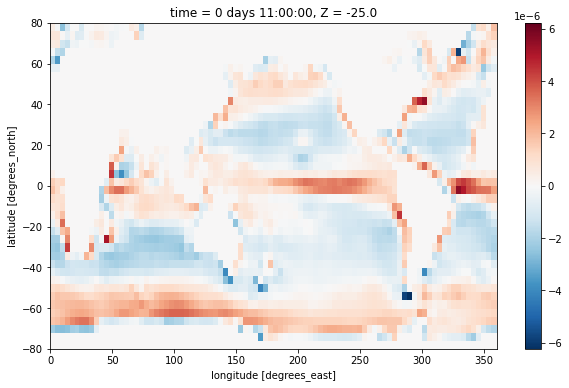
We plot this near the surface and observe the expected patern of divergence at the equator and in the subpolar regions, and convergence in the subtropical gyres.
[8]:
div_uv[0, 0].plot()
[8]:
<matplotlib.collections.QuadMesh at 0x7fec29aa8bb0>
Vorticity#
The vertical component of the vorticity is a fundamental quantity of interest in ocean circulation theory. It is defined as
On the c-grid, a finite-volume representation is given by
In xgcm, we calculate this quanity as
[9]:
zeta = (-grid.diff(ds.UVEL * ds.dxC, 'Y') + grid.diff(ds.VVEL * ds.dyC, 'X'))/ds.rAz
zeta
[9]:
<xarray.DataArray (time: 1, Z: 15, YG: 40, XG: 90)>
array([[[[-1.48332937e-08, -1.02609041e-08, -6.38644559e-09, ...,
          -2.02205257e-08, -2.36162538e-08, -2.21622898e-08],
         [ 0.00000000e+00,  0.00000000e+00,  0.00000000e+00, ...,
           0.00000000e+00,  0.00000000e+00,  0.00000000e+00],
         [ 3.81209766e-08,  3.97684836e-08,  4.13142871e-08, ...,
           1.29681979e-07,  3.34656640e-08,  3.61909045e-08],
         ...,
         [ 4.37701573e-08,  9.16013079e-08, -2.54561030e-08, ...,
           1.26603963e-08, -6.90892721e-09,  5.01466104e-08],
         [ 6.99142433e-08,  3.79757061e-08,  6.82349199e-09, ...,
           6.06992998e-08,  6.45270646e-08,  4.38413430e-08],
         [ 5.32967235e-08,  3.35858523e-08,  7.44277244e-08, ...,
          -4.63408085e-08,  1.05465695e-07, -3.87492776e-08]],

        [[-5.91518168e-09, -5.92747895e-09, -4.68231898e-09, ...,
           4.79974616e-10, -5.15723109e-09, -8.35224956e-09],
         [ 0.00000000e+00,  0.00000000e+00,  0.00000000e+00, ...,
           0.00000000e+00,  0.00000000e+00,  0.00000000e+00],
         [ 2.93285876e-08,  2.88299127e-08,  2.76142540e-08, ...,
           4.49574458e-08,  2.74702163e-08,  2.87617432e-08],
...
           0.00000000e+00,  0.00000000e+00,  0.00000000e+00],
         [ 0.00000000e+00,  0.00000000e+00,  0.00000000e+00, ...,
           0.00000000e+00,  0.00000000e+00,  0.00000000e+00],
         [ 0.00000000e+00,  0.00000000e+00,  0.00000000e+00, ...,
           0.00000000e+00,  0.00000000e+00,  0.00000000e+00]],

        [[ 0.00000000e+00,  0.00000000e+00,  0.00000000e+00, ...,
           0.00000000e+00,  0.00000000e+00,  0.00000000e+00],
         [ 0.00000000e+00,  0.00000000e+00,  0.00000000e+00, ...,
           0.00000000e+00,  0.00000000e+00,  0.00000000e+00],
         [ 0.00000000e+00,  0.00000000e+00,  0.00000000e+00, ...,
           0.00000000e+00,  0.00000000e+00,  0.00000000e+00],
         ...,
         [ 0.00000000e+00,  0.00000000e+00,  0.00000000e+00, ...,
           0.00000000e+00,  0.00000000e+00,  0.00000000e+00],
         [ 0.00000000e+00,  0.00000000e+00,  0.00000000e+00, ...,
           0.00000000e+00,  0.00000000e+00,  0.00000000e+00],
         [ 0.00000000e+00,  0.00000000e+00,  0.00000000e+00, ...,
           0.00000000e+00,  0.00000000e+00,  0.00000000e+00]]]],
      dtype=float32)
Coordinates:
  * time     (time) timedelta64[ns] 11:00:00
  * Z        (Z) float32 -25.0 -85.0 -170.0 ... -3.575e+03 -4.19e+03 -4.855e+03
  * YG       (YG) float32 -80.0 -76.0 -72.0 -68.0 -64.0 ... 64.0 68.0 72.0 76.0
  * XG       (XG) float32 0.0 4.0 8.0 12.0 16.0 ... 344.0 348.0 352.0 356.0
rAz (YG, XG) float32 3.433e+10 3.433e+10 ... 4.783e+10 4.783e+10- time: 1
- Z: 15
- YG: 40
- XG: 90
- -1.483e-08 -1.026e-08 -6.386e-09 -1.034e-08 ... 0.0 0.0 0.0 0.0
array([[[[-1.48332937e-08, -1.02609041e-08, -6.38644559e-09, ..., -2.02205257e-08, -2.36162538e-08, -2.21622898e-08], [ 0.00000000e+00, 0.00000000e+00, 0.00000000e+00, ..., 0.00000000e+00, 0.00000000e+00, 0.00000000e+00], [ 3.81209766e-08, 3.97684836e-08, 4.13142871e-08, ..., 1.29681979e-07, 3.34656640e-08, 3.61909045e-08], ..., [ 4.37701573e-08, 9.16013079e-08, -2.54561030e-08, ..., 1.26603963e-08, -6.90892721e-09, 5.01466104e-08], [ 6.99142433e-08, 3.79757061e-08, 6.82349199e-09, ..., 6.06992998e-08, 6.45270646e-08, 4.38413430e-08], [ 5.32967235e-08, 3.35858523e-08, 7.44277244e-08, ..., -4.63408085e-08, 1.05465695e-07, -3.87492776e-08]], [[-5.91518168e-09, -5.92747895e-09, -4.68231898e-09, ..., 4.79974616e-10, -5.15723109e-09, -8.35224956e-09], [ 0.00000000e+00, 0.00000000e+00, 0.00000000e+00, ..., 0.00000000e+00, 0.00000000e+00, 0.00000000e+00], [ 2.93285876e-08, 2.88299127e-08, 2.76142540e-08, ..., 4.49574458e-08, 2.74702163e-08, 2.87617432e-08], ... 0.00000000e+00, 0.00000000e+00, 0.00000000e+00], [ 0.00000000e+00, 0.00000000e+00, 0.00000000e+00, ..., 0.00000000e+00, 0.00000000e+00, 0.00000000e+00], [ 0.00000000e+00, 0.00000000e+00, 0.00000000e+00, ..., 0.00000000e+00, 0.00000000e+00, 0.00000000e+00]], [[ 0.00000000e+00, 0.00000000e+00, 0.00000000e+00, ..., 0.00000000e+00, 0.00000000e+00, 0.00000000e+00], [ 0.00000000e+00, 0.00000000e+00, 0.00000000e+00, ..., 0.00000000e+00, 0.00000000e+00, 0.00000000e+00], [ 0.00000000e+00, 0.00000000e+00, 0.00000000e+00, ..., 0.00000000e+00, 0.00000000e+00, 0.00000000e+00], ..., [ 0.00000000e+00, 0.00000000e+00, 0.00000000e+00, ..., 0.00000000e+00, 0.00000000e+00, 0.00000000e+00], [ 0.00000000e+00, 0.00000000e+00, 0.00000000e+00, ..., 0.00000000e+00, 0.00000000e+00, 0.00000000e+00], [ 0.00000000e+00, 0.00000000e+00, 0.00000000e+00, ..., 0.00000000e+00, 0.00000000e+00, 0.00000000e+00]]]], dtype=float32) - time(time)timedelta64[ns]11:00:00
- standard_name :
- time
- long_name :
- Time
- axis :
- T
- calendar :
- gregorian
array([39600000000000], dtype='timedelta64[ns]')
- Z(Z)float32-25.0 -85.0 ... -4.855e+03
- standard_name :
- depth
- long_name :
- vertical coordinate of cell center
- units :
- m
- positive :
- down
- axis :
- Z
array([ -25., -85., -170., -290., -455., -670., -935., -1250., -1615., -2030., -2495., -3010., -3575., -4190., -4855.], dtype=float32) - YG(YG)float32-80.0 -76.0 -72.0 ... 72.0 76.0
- standard_name :
- latitude_at_f_location
- long_name :
- latitude
- units :
- degrees_north
- axis :
- Y
- c_grid_axis_shift :
- -0.5
array([-80., -76., -72., -68., -64., -60., -56., -52., -48., -44., -40., -36., -32., -28., -24., -20., -16., -12., -8., -4., 0., 4., 8., 12., 16., 20., 24., 28., 32., 36., 40., 44., 48., 52., 56., 60., 64., 68., 72., 76.], dtype=float32) - XG(XG)float320.0 4.0 8.0 ... 348.0 352.0 356.0
- standard_name :
- longitude_at_f_location
- long_name :
- longitude
- units :
- degrees_east
- coordinate :
- YG XG
- axis :
- X
- c_grid_axis_shift :
- -0.5
array([ 0., 4., 8., 12., 16., 20., 24., 28., 32., 36., 40., 44., 48., 52., 56., 60., 64., 68., 72., 76., 80., 84., 88., 92., 96., 100., 104., 108., 112., 116., 120., 124., 128., 132., 136., 140., 144., 148., 152., 156., 160., 164., 168., 172., 176., 180., 184., 188., 192., 196., 200., 204., 208., 212., 216., 220., 224., 228., 232., 236., 240., 244., 248., 252., 256., 260., 264., 268., 272., 276., 280., 284., 288., 292., 296., 300., 304., 308., 312., 316., 320., 324., 328., 332., 336., 340., 344., 348., 352., 356.], dtype=float32) - rAz(YG, XG)float323.433e+10 3.433e+10 ... 4.783e+10
- standard_name :
- cell_area_at_f_location
- long_name :
- cell area
- units :
- m
- coordinate :
- YG XG
array([[3.433489e+10, 3.433489e+10, 3.433489e+10, ..., 3.433489e+10,
        3.433489e+10, 3.433489e+10],
       [4.783442e+10, 4.783442e+10, 4.783442e+10, ..., 4.783442e+10,
        4.783442e+10, 4.783442e+10],
       [6.110092e+10, 6.110092e+10, 6.110092e+10, ..., 6.110092e+10,
        6.110092e+10, 6.110092e+10],
       ...,
       [7.406974e+10, 7.406974e+10, 7.406974e+10, ..., 7.406974e+10,
        7.406974e+10, 7.406974e+10],
       [6.110092e+10, 6.110092e+10, 6.110092e+10, ..., 6.110092e+10,
        6.110092e+10, 6.110092e+10],
       [4.783442e+10, 4.783442e+10, 4.783442e+10, ..., 4.783442e+10,
        4.783442e+10, 4.783442e+10]], dtype=float32)
…which we can see is located at the YG, XG horizontal position (also commonly called the vorticity point).
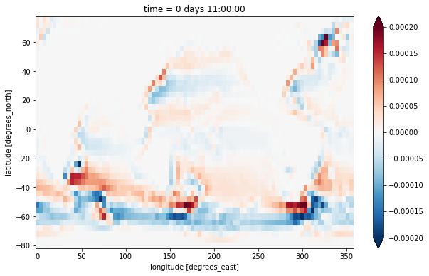
We plot the vertical integral of this quantity, i.e. the barotropic vorticity:
[10]:
zeta_bt = (zeta * ds.drF).sum(dim='Z')
zeta_bt.plot(vmax=2e-4)
[10]:
<matplotlib.collections.QuadMesh at 0x7fec28f16dc0>
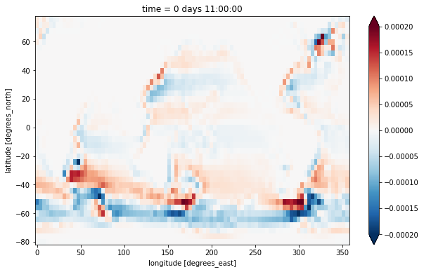
A different way to calculate the barotropic vorticity is to take the curl of the vertically integrated velocity. This formulation also allows us to incorporate the \(h\) factors representing partial cell thickness.
[11]:
u_bt = (ds.UVEL * ds.hFacW * ds.drF).sum(dim='Z')
v_bt = (ds.VVEL * ds.hFacS * ds.drF).sum(dim='Z')
zeta_bt_alt = (-grid.diff(u_bt * ds.dxC, 'Y') + grid.diff(v_bt * ds.dyC, 'X'))/ds.rAz
zeta_bt_alt.plot(vmax=2e-4)
[11]:
<matplotlib.collections.QuadMesh at 0x7fec28ac3970>
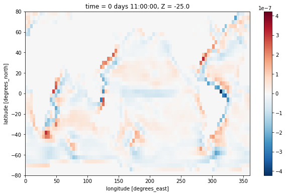
Strain#
Another interesting quantity is the horizontal strain, defined as
On the c-grid, a finite-volume representation is given by
[12]:
strain = (grid.diff(ds.UVEL * ds.dyG, 'X') - grid.diff(ds.VVEL * ds.dxG, 'Y')) / ds.rA
strain[0,0].plot()
[12]:
<matplotlib.collections.QuadMesh at 0x7fec28f2d6a0>
Barotropic Transport Streamfunction#
We can use the barotropic velocity to calcuate the barotropic transport streamfunction, defined via
We calculate this by integrating \(u_{bt}\) along the Y axis using the grid object’s cumsum method:
[13]:
psi = grid.cumsum(-u_bt * ds.dyG, 'Y', boundary='fill')
psi
[13]:
<xarray.DataArray (time: 1, YG: 40, XG: 90)>
array([[[ 0.00000000e+00,  0.00000000e+00,  0.00000000e+00, ...,
          0.00000000e+00,  0.00000000e+00,  0.00000000e+00],
        [-0.00000000e+00, -0.00000000e+00, -0.00000000e+00, ...,
         -0.00000000e+00, -0.00000000e+00, -0.00000000e+00],
        [-0.00000000e+00, -0.00000000e+00, -0.00000000e+00, ...,
         -0.00000000e+00, -0.00000000e+00, -0.00000000e+00],
        ...,
        [-1.06634920e+08, -1.06666912e+08, -1.05922952e+08, ...,
         -1.07724152e+08, -1.07341128e+08, -1.06941400e+08],
        [-1.07050680e+08, -1.06612056e+08, -1.06356232e+08, ...,
         -1.07048232e+08, -1.07335792e+08, -1.07102304e+08],
        [-1.05933672e+08, -1.05922800e+08, -1.05856504e+08, ...,
         -1.05376272e+08, -1.05493376e+08, -1.05632128e+08]]],
      dtype=float32)
Coordinates:
  * time     (time) timedelta64[ns] 11:00:00
  * YG       (YG) float32 -80.0 -76.0 -72.0 -68.0 -64.0 ... 64.0 68.0 72.0 76.0
* XG (XG) float32 0.0 4.0 8.0 12.0 16.0 ... 344.0 348.0 352.0 356.0- time: 1
- YG: 40
- XG: 90
- 0.0 0.0 0.0 0.0 0.0 ... -1.054e+08 -1.054e+08 -1.055e+08 -1.056e+08
array([[[ 0.00000000e+00, 0.00000000e+00, 0.00000000e+00, ..., 0.00000000e+00, 0.00000000e+00, 0.00000000e+00], [-0.00000000e+00, -0.00000000e+00, -0.00000000e+00, ..., -0.00000000e+00, -0.00000000e+00, -0.00000000e+00], [-0.00000000e+00, -0.00000000e+00, -0.00000000e+00, ..., -0.00000000e+00, -0.00000000e+00, -0.00000000e+00], ..., [-1.06634920e+08, -1.06666912e+08, -1.05922952e+08, ..., -1.07724152e+08, -1.07341128e+08, -1.06941400e+08], [-1.07050680e+08, -1.06612056e+08, -1.06356232e+08, ..., -1.07048232e+08, -1.07335792e+08, -1.07102304e+08], [-1.05933672e+08, -1.05922800e+08, -1.05856504e+08, ..., -1.05376272e+08, -1.05493376e+08, -1.05632128e+08]]], dtype=float32) - time(time)timedelta64[ns]11:00:00
- standard_name :
- time
- long_name :
- Time
- axis :
- T
- calendar :
- gregorian
array([39600000000000], dtype='timedelta64[ns]')
- YG(YG)float32-80.0 -76.0 -72.0 ... 72.0 76.0
- standard_name :
- latitude_at_f_location
- long_name :
- latitude
- units :
- degrees_north
- axis :
- Y
- c_grid_axis_shift :
- -0.5
array([-80., -76., -72., -68., -64., -60., -56., -52., -48., -44., -40., -36., -32., -28., -24., -20., -16., -12., -8., -4., 0., 4., 8., 12., 16., 20., 24., 28., 32., 36., 40., 44., 48., 52., 56., 60., 64., 68., 72., 76.], dtype=float32) - XG(XG)float320.0 4.0 8.0 ... 348.0 352.0 356.0
- standard_name :
- longitude_at_f_location
- long_name :
- longitude
- units :
- degrees_east
- coordinate :
- YG XG
- axis :
- X
- c_grid_axis_shift :
- -0.5
array([  0.,   4.,   8.,  12.,  16.,  20.,  24.,  28.,  32.,  36.,  40.,  44.,
        48.,  52.,  56.,  60.,  64.,  68.,  72.,  76.,  80.,  84.,  88.,  92.,
        96., 100., 104., 108., 112., 116., 120., 124., 128., 132., 136., 140.,
       144., 148., 152., 156., 160., 164., 168., 172., 176., 180., 184., 188.,
       192., 196., 200., 204., 208., 212., 216., 220., 224., 228., 232., 236.,
       240., 244., 248., 252., 256., 260., 264., 268., 272., 276., 280., 284.,
       288., 292., 296., 300., 304., 308., 312., 316., 320., 324., 328., 332.,
       336., 340., 344., 348., 352., 356.], dtype=float32)
We see that xgcm automatically shifted the Y-axis position from center (YC) to left (YG) during the cumsum operation.
We convert to sverdrups and plot with a contour plot.
[14]:
(psi[0] / 1e6).plot.contourf(levels=np.arange(-160, 40, 5))
[14]:
<matplotlib.contour.QuadContourSet at 0x7fec294e19a0>
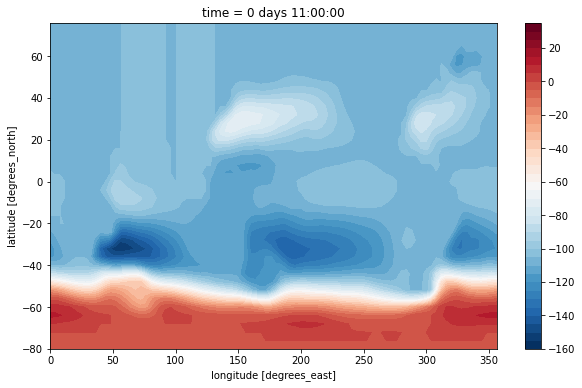
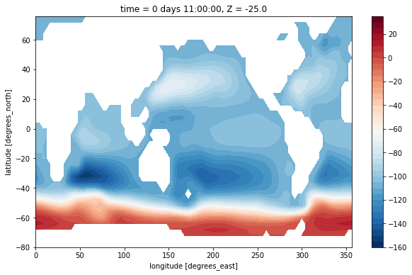
This doesn’t look nice because it lacks a suitable land mask. The dataset has no mask provided for the vorticity point. But we can build one with xgcm!
[15]:
maskZ = grid.interp(ds.hFacS, 'X')
(psi[0] / 1e6).where(maskZ[0]).plot.contourf(levels=np.arange(-160, 40, 5))
[15]:
<matplotlib.contour.QuadContourSet at 0x7fec29ce21f0>
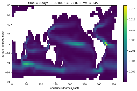
Kinetic Energy#
Finally, we plot the kinetic energy \(1/2 (u^2 + v^2)\) by interpoloting both quantities the cell center point.
[16]:
ke = 0.5*(grid.interp((ds.UVEL*ds.hFacW)**2, 'X') + grid.interp((ds.VVEL*ds.hFacS)**2, 'Y'))
ke[0,0].where(ds.maskC[0]).plot()
[16]:
<matplotlib.collections.QuadMesh at 0x7fec2911cd90>
[ ]:
[ ]:
[ ]:
[ ]: