MITgcm ECCOv4 Example#
This Jupyter notebook demonstrates how to use xarray and xgcm to analyze data from the ECCO v4r3 ocean state estimate.
This notebook can be viewed and executed interactively viaPangeo Gallery.
First we import our standard python packages:
[1]:
import xarray as xr
import numpy as np
from matplotlib import pyplot as plt
%matplotlib inline
Load the data#
The ECCOv4r3 data was converted from its raw MDS (.data / .meta file) format to zarr format, using the xmitgcm package. Zarr is a powerful data storage format that can be thought of as an alternative to HDF. In contrast to HDF, zarr works very well with cloud object storage. Zarr is currently useable in python, java, C++, and julia. It is likely that zarr will form the basis of the next major version of the netCDF library.
If you’re curious, here are some resources to learn more about zarr: - https://zarr.readthedocs.io/en/stable/tutorial.html - https://speakerdeck.com/rabernat/pangeo-zarr-cloud-data-storage - https://mrocklin.github.com/blog/work/2018/02/06/hdf-in-the-cloud
The ECCO zarr data currently lives in Google Cloud Storage as part of the Pangeo Data Catalog. This means we can open the whole dataset using one line of code.
This takes a bit of time to run because the metadata must be downloaded and parsed. The type of object returned is an Xarray dataset.
[2]:
import intake
cat = intake.open_catalog("https://raw.githubusercontent.com/pangeo-data/pangeo-datastore/master/intake-catalogs/ocean.yaml")
ds = cat.ECCOv4r3.to_dask()
ds
[2]:
<xarray.Dataset>
Dimensions:    (face: 13, i: 90, i_g: 90, j: 90, j_g: 90, k: 50, k_l: 50, k_p1: 51, k_u: 50, time: 288, time_snp: 287)
Coordinates:
    Depth      (face, j, i) float32 dask.array<chunksize=(13, 90, 90), meta=np.ndarray>
    PHrefC     (k) float32 dask.array<chunksize=(50,), meta=np.ndarray>
    PHrefF     (k_p1) float32 dask.array<chunksize=(51,), meta=np.ndarray>
    XC         (face, j, i) float32 dask.array<chunksize=(13, 90, 90), meta=np.ndarray>
    XG         (face, j_g, i_g) float32 dask.array<chunksize=(13, 90, 90), meta=np.ndarray>
    YC         (face, j, i) float32 dask.array<chunksize=(13, 90, 90), meta=np.ndarray>
    YG         (face, j_g, i_g) float32 dask.array<chunksize=(13, 90, 90), meta=np.ndarray>
    Z          (k) float32 dask.array<chunksize=(50,), meta=np.ndarray>
    Zl         (k_l) float32 dask.array<chunksize=(50,), meta=np.ndarray>
    Zp1        (k_p1) float32 dask.array<chunksize=(51,), meta=np.ndarray>
    Zu         (k_u) float32 dask.array<chunksize=(50,), meta=np.ndarray>
    drC        (k_p1) float32 dask.array<chunksize=(51,), meta=np.ndarray>
    drF        (k) float32 dask.array<chunksize=(50,), meta=np.ndarray>
    dxC        (face, j, i_g) float32 dask.array<chunksize=(13, 90, 90), meta=np.ndarray>
    dxG        (face, j_g, i) float32 dask.array<chunksize=(13, 90, 90), meta=np.ndarray>
    dyC        (face, j_g, i) float32 dask.array<chunksize=(13, 90, 90), meta=np.ndarray>
    dyG        (face, j, i_g) float32 dask.array<chunksize=(13, 90, 90), meta=np.ndarray>
  * face       (face) int64 0 1 2 3 4 5 6 7 8 9 10 11 12
    hFacC      (k, face, j, i) float32 dask.array<chunksize=(50, 13, 90, 90), meta=np.ndarray>
    hFacS      (k, face, j_g, i) float32 dask.array<chunksize=(50, 13, 90, 90), meta=np.ndarray>
    hFacW      (k, face, j, i_g) float32 dask.array<chunksize=(50, 13, 90, 90), meta=np.ndarray>
  * i          (i) int64 0 1 2 3 4 5 6 7 8 9 ... 80 81 82 83 84 85 86 87 88 89
  * i_g        (i_g) int64 0 1 2 3 4 5 6 7 8 9 ... 80 81 82 83 84 85 86 87 88 89
    iter       (time) int64 dask.array<chunksize=(1,), meta=np.ndarray>
    iter_snp   (time_snp) int64 dask.array<chunksize=(1,), meta=np.ndarray>
  * j          (j) int64 0 1 2 3 4 5 6 7 8 9 ... 80 81 82 83 84 85 86 87 88 89
  * j_g        (j_g) int64 0 1 2 3 4 5 6 7 8 9 ... 80 81 82 83 84 85 86 87 88 89
  * k          (k) int64 0 1 2 3 4 5 6 7 8 9 ... 40 41 42 43 44 45 46 47 48 49
  * k_l        (k_l) int64 0 1 2 3 4 5 6 7 8 9 ... 40 41 42 43 44 45 46 47 48 49
  * k_p1       (k_p1) int64 0 1 2 3 4 5 6 7 8 9 ... 42 43 44 45 46 47 48 49 50
  * k_u        (k_u) int64 0 1 2 3 4 5 6 7 8 9 ... 40 41 42 43 44 45 46 47 48 49
    rA         (face, j, i) float32 dask.array<chunksize=(13, 90, 90), meta=np.ndarray>
    rAs        (face, j_g, i) float32 dask.array<chunksize=(13, 90, 90), meta=np.ndarray>
    rAw        (face, j, i_g) float32 dask.array<chunksize=(13, 90, 90), meta=np.ndarray>
    rAz        (face, j_g, i_g) float32 dask.array<chunksize=(13, 90, 90), meta=np.ndarray>
  * time       (time) datetime64[ns] 1992-01-15 1992-02-13 ... 2015-12-14
  * time_snp   (time_snp) datetime64[ns] 1992-02-01 1992-03-01 ... 2015-12-01
Data variables:
    ADVr_SLT   (time, k_l, face, j, i) float32 dask.array<chunksize=(1, 50, 13, 90, 90), meta=np.ndarray>
    ADVr_TH    (time, k_l, face, j, i) float32 dask.array<chunksize=(1, 50, 13, 90, 90), meta=np.ndarray>
    ADVx_SLT   (time, k, face, j, i_g) float32 dask.array<chunksize=(1, 50, 13, 90, 90), meta=np.ndarray>
    ADVx_TH    (time, k, face, j, i_g) float32 dask.array<chunksize=(1, 50, 13, 90, 90), meta=np.ndarray>
    ADVy_SLT   (time, k, face, j_g, i) float32 dask.array<chunksize=(1, 50, 13, 90, 90), meta=np.ndarray>
    ADVy_TH    (time, k, face, j_g, i) float32 dask.array<chunksize=(1, 50, 13, 90, 90), meta=np.ndarray>
    DFrE_SLT   (time, k_l, face, j, i) float32 dask.array<chunksize=(1, 50, 13, 90, 90), meta=np.ndarray>
    DFrE_TH    (time, k_l, face, j, i) float32 dask.array<chunksize=(1, 50, 13, 90, 90), meta=np.ndarray>
    DFrI_SLT   (time, k_l, face, j, i) float32 dask.array<chunksize=(1, 50, 13, 90, 90), meta=np.ndarray>
    DFrI_TH    (time, k_l, face, j, i) float32 dask.array<chunksize=(1, 50, 13, 90, 90), meta=np.ndarray>
    DFxE_SLT   (time, k, face, j, i_g) float32 dask.array<chunksize=(1, 50, 13, 90, 90), meta=np.ndarray>
    DFxE_TH    (time, k, face, j, i_g) float32 dask.array<chunksize=(1, 50, 13, 90, 90), meta=np.ndarray>
    DFyE_SLT   (time, k, face, j_g, i) float32 dask.array<chunksize=(1, 50, 13, 90, 90), meta=np.ndarray>
    DFyE_TH    (time, k, face, j_g, i) float32 dask.array<chunksize=(1, 50, 13, 90, 90), meta=np.ndarray>
    ETAN       (time, face, j, i) float32 dask.array<chunksize=(1, 13, 90, 90), meta=np.ndarray>
    ETAN_snp   (time_snp, face, j, i) float32 dask.array<chunksize=(1, 13, 90, 90), meta=np.ndarray>
    GEOFLX     (face, j, i) float32 dask.array<chunksize=(7, 90, 90), meta=np.ndarray>
    MXLDEPTH   (time, face, j, i) float32 dask.array<chunksize=(1, 1, 90, 90), meta=np.ndarray>
    SALT       (time, k, face, j, i) float32 dask.array<chunksize=(1, 50, 13, 90, 90), meta=np.ndarray>
    SALT_snp   (time_snp, k, face, j, i) float32 dask.array<chunksize=(1, 50, 13, 90, 90), meta=np.ndarray>
    SFLUX      (time, face, j, i) float32 dask.array<chunksize=(1, 13, 90, 90), meta=np.ndarray>
    TFLUX      (time, face, j, i) float32 dask.array<chunksize=(1, 13, 90, 90), meta=np.ndarray>
    THETA      (time, k, face, j, i) float32 dask.array<chunksize=(1, 50, 13, 90, 90), meta=np.ndarray>
    THETA_snp  (time_snp, k, face, j, i) float32 dask.array<chunksize=(1, 50, 13, 90, 90), meta=np.ndarray>
    UVELMASS   (time, k, face, j, i_g) float32 dask.array<chunksize=(1, 50, 13, 90, 90), meta=np.ndarray>
    UVELSTAR   (time, k, face, j, i_g) float32 dask.array<chunksize=(1, 50, 1, 90, 90), meta=np.ndarray>
    VVELMASS   (time, k, face, j_g, i) float32 dask.array<chunksize=(1, 50, 13, 90, 90), meta=np.ndarray>
    VVELSTAR   (time, k, face, j_g, i) float32 dask.array<chunksize=(1, 50, 1, 90, 90), meta=np.ndarray>
    WVELMASS   (time, k_l, face, j, i) float32 dask.array<chunksize=(1, 50, 13, 90, 90), meta=np.ndarray>
    WVELSTAR   (time, k_l, face, j, i) float32 dask.array<chunksize=(1, 50, 1, 90, 90), meta=np.ndarray>
    oceFWflx   (time, face, j, i) float32 dask.array<chunksize=(1, 13, 90, 90), meta=np.ndarray>
    oceQsw     (time, face, j, i) float32 dask.array<chunksize=(1, 13, 90, 90), meta=np.ndarray>
    oceSPtnd   (time, k, face, j, i) float32 dask.array<chunksize=(1, 50, 13, 90, 90), meta=np.ndarray>
    oceTAUX    (time, face, j, i_g) float32 dask.array<chunksize=(1, 1, 90, 90), meta=np.ndarray>
oceTAUY (time, face, j_g, i) float32 dask.array<chunksize=(1, 1, 90, 90), meta=np.ndarray>- face: 13
- i: 90
- i_g: 90
- j: 90
- j_g: 90
- k: 50
- k_l: 50
- k_p1: 51
- k_u: 50
- time: 288
- time_snp: 287
- Depth(face, j, i)float32dask.array<chunksize=(13, 90, 90), meta=np.ndarray>
- coordinate :
- XC YC
- long_name :
- ocean depth
- standard_name :
- ocean_depth
- units :
- m
Array Chunk Bytes 421.20 kB 421.20 kB Shape (13, 90, 90) (13, 90, 90) Count 2 Tasks 1 Chunks Type float32 numpy.ndarray - PHrefC(k)float32dask.array<chunksize=(50,), meta=np.ndarray>
- long_name :
- Reference Hydrostatic Pressure
- standard_name :
- cell_reference_pressure
- units :
- m2 s-2
Array Chunk Bytes 200 B 200 B Shape (50,) (50,) Count 2 Tasks 1 Chunks Type float32 numpy.ndarray - PHrefF(k_p1)float32dask.array<chunksize=(51,), meta=np.ndarray>
- long_name :
- Reference Hydrostatic Pressure
- standard_name :
- cell_reference_pressure
- units :
- m2 s-2
Array Chunk Bytes 204 B 204 B Shape (51,) (51,) Count 2 Tasks 1 Chunks Type float32 numpy.ndarray - XC(face, j, i)float32dask.array<chunksize=(13, 90, 90), meta=np.ndarray>
- coordinate :
- YC XC
- long_name :
- longitude
- standard_name :
- longitude
- units :
- degrees_east
Array Chunk Bytes 421.20 kB 421.20 kB Shape (13, 90, 90) (13, 90, 90) Count 2 Tasks 1 Chunks Type float32 numpy.ndarray - XG(face, j_g, i_g)float32dask.array<chunksize=(13, 90, 90), meta=np.ndarray>
- coordinate :
- YG XG
- long_name :
- longitude
- standard_name :
- longitude_at_f_location
- units :
- degrees_east
Array Chunk Bytes 421.20 kB 421.20 kB Shape (13, 90, 90) (13, 90, 90) Count 2 Tasks 1 Chunks Type float32 numpy.ndarray - YC(face, j, i)float32dask.array<chunksize=(13, 90, 90), meta=np.ndarray>
- coordinate :
- YC XC
- long_name :
- latitude
- standard_name :
- latitude
- units :
- degrees_north
Array Chunk Bytes 421.20 kB 421.20 kB Shape (13, 90, 90) (13, 90, 90) Count 2 Tasks 1 Chunks Type float32 numpy.ndarray - YG(face, j_g, i_g)float32dask.array<chunksize=(13, 90, 90), meta=np.ndarray>
- long_name :
- latitude
- standard_name :
- latitude_at_f_location
- units :
- degrees_north
Array Chunk Bytes 421.20 kB 421.20 kB Shape (13, 90, 90) (13, 90, 90) Count 2 Tasks 1 Chunks Type float32 numpy.ndarray - Z(k)float32dask.array<chunksize=(50,), meta=np.ndarray>
- long_name :
- vertical coordinate of cell center
- positive :
- down
- standard_name :
- depth
- units :
- m
Array Chunk Bytes 200 B 200 B Shape (50,) (50,) Count 2 Tasks 1 Chunks Type float32 numpy.ndarray - Zl(k_l)float32dask.array<chunksize=(50,), meta=np.ndarray>
- long_name :
- vertical coordinate of upper cell interface
- positive :
- down
- standard_name :
- depth_at_upper_w_location
- units :
- m
Array Chunk Bytes 200 B 200 B Shape (50,) (50,) Count 2 Tasks 1 Chunks Type float32 numpy.ndarray - Zp1(k_p1)float32dask.array<chunksize=(51,), meta=np.ndarray>
- long_name :
- vertical coordinate of cell interface
- positive :
- down
- standard_name :
- depth_at_w_location
- units :
- m
Array Chunk Bytes 204 B 204 B Shape (51,) (51,) Count 2 Tasks 1 Chunks Type float32 numpy.ndarray - Zu(k_u)float32dask.array<chunksize=(50,), meta=np.ndarray>
- long_name :
- vertical coordinate of lower cell interface
- positive :
- down
- standard_name :
- depth_at_lower_w_location
- units :
- m
Array Chunk Bytes 200 B 200 B Shape (50,) (50,) Count 2 Tasks 1 Chunks Type float32 numpy.ndarray - drC(k_p1)float32dask.array<chunksize=(51,), meta=np.ndarray>
- long_name :
- cell z size
- standard_name :
- cell_z_size_at_w_location
- units :
- m
Array Chunk Bytes 204 B 204 B Shape (51,) (51,) Count 2 Tasks 1 Chunks Type float32 numpy.ndarray - drF(k)float32dask.array<chunksize=(50,), meta=np.ndarray>
- long_name :
- cell z size
- standard_name :
- cell_z_size
- units :
- m
Array Chunk Bytes 200 B 200 B Shape (50,) (50,) Count 2 Tasks 1 Chunks Type float32 numpy.ndarray - dxC(face, j, i_g)float32dask.array<chunksize=(13, 90, 90), meta=np.ndarray>
- coordinate :
- YC XG
- long_name :
- cell x size
- standard_name :
- cell_x_size_at_u_location
- units :
- m
Array Chunk Bytes 421.20 kB 421.20 kB Shape (13, 90, 90) (13, 90, 90) Count 2 Tasks 1 Chunks Type float32 numpy.ndarray - dxG(face, j_g, i)float32dask.array<chunksize=(13, 90, 90), meta=np.ndarray>
- coordinate :
- YG XC
- long_name :
- cell x size
- standard_name :
- cell_x_size_at_v_location
- units :
- m
Array Chunk Bytes 421.20 kB 421.20 kB Shape (13, 90, 90) (13, 90, 90) Count 2 Tasks 1 Chunks Type float32 numpy.ndarray - dyC(face, j_g, i)float32dask.array<chunksize=(13, 90, 90), meta=np.ndarray>
- coordinate :
- YG XC
- long_name :
- cell y size
- standard_name :
- cell_y_size_at_v_location
- units :
- m
Array Chunk Bytes 421.20 kB 421.20 kB Shape (13, 90, 90) (13, 90, 90) Count 2 Tasks 1 Chunks Type float32 numpy.ndarray - dyG(face, j, i_g)float32dask.array<chunksize=(13, 90, 90), meta=np.ndarray>
- coordinate :
- YC XG
- long_name :
- cell y size
- standard_name :
- cell_y_size_at_u_location
- units :
- m
Array Chunk Bytes 421.20 kB 421.20 kB Shape (13, 90, 90) (13, 90, 90) Count 2 Tasks 1 Chunks Type float32 numpy.ndarray - face(face)int640 1 2 3 4 5 6 7 8 9 10 11 12
- standard_name :
- face_index
array([ 0, 1, 2, 3, 4, 5, 6, 7, 8, 9, 10, 11, 12])
- hFacC(k, face, j, i)float32dask.array<chunksize=(50, 13, 90, 90), meta=np.ndarray>
- long_name :
- vertical fraction of open cell
- standard_name :
- cell_vertical_fraction
Array Chunk Bytes 21.06 MB 21.06 MB Shape (50, 13, 90, 90) (50, 13, 90, 90) Count 2 Tasks 1 Chunks Type float32 numpy.ndarray - hFacS(k, face, j_g, i)float32dask.array<chunksize=(50, 13, 90, 90), meta=np.ndarray>
- long_name :
- vertical fraction of open cell
- standard_name :
- cell_vertical_fraction_at_v_location
Array Chunk Bytes 21.06 MB 21.06 MB Shape (50, 13, 90, 90) (50, 13, 90, 90) Count 2 Tasks 1 Chunks Type float32 numpy.ndarray - hFacW(k, face, j, i_g)float32dask.array<chunksize=(50, 13, 90, 90), meta=np.ndarray>
- long_name :
- vertical fraction of open cell
- standard_name :
- cell_vertical_fraction_at_u_location
Array Chunk Bytes 21.06 MB 21.06 MB Shape (50, 13, 90, 90) (50, 13, 90, 90) Count 2 Tasks 1 Chunks Type float32 numpy.ndarray - i(i)int640 1 2 3 4 5 6 ... 84 85 86 87 88 89
- axis :
- X
- long_name :
- x-dimension of the t grid
- standard_name :
- x_grid_index
- swap_dim :
- XC
array([ 0, 1, 2, 3, 4, 5, 6, 7, 8, 9, 10, 11, 12, 13, 14, 15, 16, 17, 18, 19, 20, 21, 22, 23, 24, 25, 26, 27, 28, 29, 30, 31, 32, 33, 34, 35, 36, 37, 38, 39, 40, 41, 42, 43, 44, 45, 46, 47, 48, 49, 50, 51, 52, 53, 54, 55, 56, 57, 58, 59, 60, 61, 62, 63, 64, 65, 66, 67, 68, 69, 70, 71, 72, 73, 74, 75, 76, 77, 78, 79, 80, 81, 82, 83, 84, 85, 86, 87, 88, 89]) - i_g(i_g)int640 1 2 3 4 5 6 ... 84 85 86 87 88 89
- axis :
- X
- c_grid_axis_shift :
- -0.5
- long_name :
- x-dimension of the u grid
- standard_name :
- x_grid_index_at_u_location
- swap_dim :
- XG
array([ 0, 1, 2, 3, 4, 5, 6, 7, 8, 9, 10, 11, 12, 13, 14, 15, 16, 17, 18, 19, 20, 21, 22, 23, 24, 25, 26, 27, 28, 29, 30, 31, 32, 33, 34, 35, 36, 37, 38, 39, 40, 41, 42, 43, 44, 45, 46, 47, 48, 49, 50, 51, 52, 53, 54, 55, 56, 57, 58, 59, 60, 61, 62, 63, 64, 65, 66, 67, 68, 69, 70, 71, 72, 73, 74, 75, 76, 77, 78, 79, 80, 81, 82, 83, 84, 85, 86, 87, 88, 89]) - iter(time)int64dask.array<chunksize=(1,), meta=np.ndarray>
- long_name :
- model timestep number
- standard_name :
- timestep
Array Chunk Bytes 2.30 kB 8 B Shape (288,) (1,) Count 289 Tasks 288 Chunks Type int64 numpy.ndarray - iter_snp(time_snp)int64dask.array<chunksize=(1,), meta=np.ndarray>
- long_name :
- model timestep number
- standard_name :
- timestep
Array Chunk Bytes 2.30 kB 8 B Shape (287,) (1,) Count 288 Tasks 287 Chunks Type int64 numpy.ndarray - j(j)int640 1 2 3 4 5 6 ... 84 85 86 87 88 89
- axis :
- Y
- long_name :
- y-dimension of the t grid
- standard_name :
- y_grid_index
- swap_dim :
- YC
array([ 0, 1, 2, 3, 4, 5, 6, 7, 8, 9, 10, 11, 12, 13, 14, 15, 16, 17, 18, 19, 20, 21, 22, 23, 24, 25, 26, 27, 28, 29, 30, 31, 32, 33, 34, 35, 36, 37, 38, 39, 40, 41, 42, 43, 44, 45, 46, 47, 48, 49, 50, 51, 52, 53, 54, 55, 56, 57, 58, 59, 60, 61, 62, 63, 64, 65, 66, 67, 68, 69, 70, 71, 72, 73, 74, 75, 76, 77, 78, 79, 80, 81, 82, 83, 84, 85, 86, 87, 88, 89]) - j_g(j_g)int640 1 2 3 4 5 6 ... 84 85 86 87 88 89
- axis :
- Y
- c_grid_axis_shift :
- -0.5
- long_name :
- y-dimension of the v grid
- standard_name :
- y_grid_index_at_v_location
- swap_dim :
- YG
array([ 0, 1, 2, 3, 4, 5, 6, 7, 8, 9, 10, 11, 12, 13, 14, 15, 16, 17, 18, 19, 20, 21, 22, 23, 24, 25, 26, 27, 28, 29, 30, 31, 32, 33, 34, 35, 36, 37, 38, 39, 40, 41, 42, 43, 44, 45, 46, 47, 48, 49, 50, 51, 52, 53, 54, 55, 56, 57, 58, 59, 60, 61, 62, 63, 64, 65, 66, 67, 68, 69, 70, 71, 72, 73, 74, 75, 76, 77, 78, 79, 80, 81, 82, 83, 84, 85, 86, 87, 88, 89]) - k(k)int640 1 2 3 4 5 6 ... 44 45 46 47 48 49
- axis :
- Z
- long_name :
- z-dimension of the t grid
- standard_name :
- z_grid_index
- swap_dim :
- Z
array([ 0, 1, 2, 3, 4, 5, 6, 7, 8, 9, 10, 11, 12, 13, 14, 15, 16, 17, 18, 19, 20, 21, 22, 23, 24, 25, 26, 27, 28, 29, 30, 31, 32, 33, 34, 35, 36, 37, 38, 39, 40, 41, 42, 43, 44, 45, 46, 47, 48, 49]) - k_l(k_l)int640 1 2 3 4 5 6 ... 44 45 46 47 48 49
- axis :
- Z
- c_grid_axis_shift :
- -0.5
- long_name :
- z-dimension of the w grid
- standard_name :
- z_grid_index_at_upper_w_location
- swap_dim :
- Zl
array([ 0, 1, 2, 3, 4, 5, 6, 7, 8, 9, 10, 11, 12, 13, 14, 15, 16, 17, 18, 19, 20, 21, 22, 23, 24, 25, 26, 27, 28, 29, 30, 31, 32, 33, 34, 35, 36, 37, 38, 39, 40, 41, 42, 43, 44, 45, 46, 47, 48, 49]) - k_p1(k_p1)int640 1 2 3 4 5 6 ... 45 46 47 48 49 50
- axis :
- Z
- c_grid_axis_shift :
- [-0.5, 0.5]
- long_name :
- z-dimension of the w grid
- standard_name :
- z_grid_index_at_w_location
- swap_dim :
- Zp1
array([ 0, 1, 2, 3, 4, 5, 6, 7, 8, 9, 10, 11, 12, 13, 14, 15, 16, 17, 18, 19, 20, 21, 22, 23, 24, 25, 26, 27, 28, 29, 30, 31, 32, 33, 34, 35, 36, 37, 38, 39, 40, 41, 42, 43, 44, 45, 46, 47, 48, 49, 50]) - k_u(k_u)int640 1 2 3 4 5 6 ... 44 45 46 47 48 49
- axis :
- Z
- c_grid_axis_shift :
- 0.5
- long_name :
- z-dimension of the w grid
- standard_name :
- z_grid_index_at_lower_w_location
- swap_dim :
- Zu
array([ 0, 1, 2, 3, 4, 5, 6, 7, 8, 9, 10, 11, 12, 13, 14, 15, 16, 17, 18, 19, 20, 21, 22, 23, 24, 25, 26, 27, 28, 29, 30, 31, 32, 33, 34, 35, 36, 37, 38, 39, 40, 41, 42, 43, 44, 45, 46, 47, 48, 49]) - rA(face, j, i)float32dask.array<chunksize=(13, 90, 90), meta=np.ndarray>
- coordinate :
- YC XC
- long_name :
- cell area
- standard_name :
- cell_area
- units :
- m2
Array Chunk Bytes 421.20 kB 421.20 kB Shape (13, 90, 90) (13, 90, 90) Count 2 Tasks 1 Chunks Type float32 numpy.ndarray - rAs(face, j_g, i)float32dask.array<chunksize=(13, 90, 90), meta=np.ndarray>
- long_name :
- cell area
- standard_name :
- cell_area_at_v_location
- units :
- m2
Array Chunk Bytes 421.20 kB 421.20 kB Shape (13, 90, 90) (13, 90, 90) Count 2 Tasks 1 Chunks Type float32 numpy.ndarray - rAw(face, j, i_g)float32dask.array<chunksize=(13, 90, 90), meta=np.ndarray>
- coordinate :
- YG XC
- long_name :
- cell area
- standard_name :
- cell_area_at_u_location
- units :
- m2
Array Chunk Bytes 421.20 kB 421.20 kB Shape (13, 90, 90) (13, 90, 90) Count 2 Tasks 1 Chunks Type float32 numpy.ndarray - rAz(face, j_g, i_g)float32dask.array<chunksize=(13, 90, 90), meta=np.ndarray>
- coordinate :
- YG XG
- long_name :
- cell area
- standard_name :
- cell_area_at_f_location
- units :
- m
Array Chunk Bytes 421.20 kB 421.20 kB Shape (13, 90, 90) (13, 90, 90) Count 2 Tasks 1 Chunks Type float32 numpy.ndarray - time(time)datetime64[ns]1992-01-15 ... 2015-12-14
- axis :
- T
- long_name :
- Time
- standard_name :
- time
array(['1992-01-15T00:00:00.000000000', '1992-02-13T00:00:00.000000000', '1992-03-15T00:00:00.000000000', ..., '2015-10-15T00:00:00.000000000', '2015-11-14T00:00:00.000000000', '2015-12-14T00:00:00.000000000'], dtype='datetime64[ns]') - time_snp(time_snp)datetime64[ns]1992-02-01 ... 2015-12-01
- axis :
- T
- c_grid_axis_shift :
- 0.5
- long_name :
- Time
- standard_name :
- time
array(['1992-02-01T00:00:00.000000000', '1992-03-01T00:00:00.000000000',
       '1992-04-01T00:00:00.000000000', ..., '2015-10-01T00:00:00.000000000',
       '2015-11-01T00:00:00.000000000', '2015-12-01T00:00:00.000000000'],
      dtype='datetime64[ns]')
- ADVr_SLT(time, k_l, face, j, i)float32dask.array<chunksize=(1, 50, 13, 90, 90), meta=np.ndarray>
- long_name :
- Vertical Advective Flux of Salinity
- standard_name :
- ADVr_SLT
- units :
- psu.m^3/s
Array Chunk Bytes 6.07 GB 21.06 MB Shape (288, 50, 13, 90, 90) (1, 50, 13, 90, 90) Count 289 Tasks 288 Chunks Type float32 numpy.ndarray - ADVr_TH(time, k_l, face, j, i)float32dask.array<chunksize=(1, 50, 13, 90, 90), meta=np.ndarray>
- long_name :
- Vertical Advective Flux of Pot.Temperature
- standard_name :
- ADVr_TH
- units :
- degC.m^3/s
Array Chunk Bytes 6.07 GB 21.06 MB Shape (288, 50, 13, 90, 90) (1, 50, 13, 90, 90) Count 289 Tasks 288 Chunks Type float32 numpy.ndarray - ADVx_SLT(time, k, face, j, i_g)float32dask.array<chunksize=(1, 50, 13, 90, 90), meta=np.ndarray>
- long_name :
- Zonal Advective Flux of Salinity
- mate :
- ADVy_SLT
- standard_name :
- ADVx_SLT
- units :
- psu.m^3/s
Array Chunk Bytes 6.07 GB 21.06 MB Shape (288, 50, 13, 90, 90) (1, 50, 13, 90, 90) Count 289 Tasks 288 Chunks Type float32 numpy.ndarray - ADVx_TH(time, k, face, j, i_g)float32dask.array<chunksize=(1, 50, 13, 90, 90), meta=np.ndarray>
- long_name :
- Zonal Advective Flux of Pot.Temperature
- mate :
- ADVy_TH
- standard_name :
- ADVx_TH
- units :
- degC.m^3/s
Array Chunk Bytes 6.07 GB 21.06 MB Shape (288, 50, 13, 90, 90) (1, 50, 13, 90, 90) Count 289 Tasks 288 Chunks Type float32 numpy.ndarray - ADVy_SLT(time, k, face, j_g, i)float32dask.array<chunksize=(1, 50, 13, 90, 90), meta=np.ndarray>
- long_name :
- Meridional Advective Flux of Salinity
- mate :
- ADVx_SLT
- standard_name :
- ADVy_SLT
- units :
- psu.m^3/s
Array Chunk Bytes 6.07 GB 21.06 MB Shape (288, 50, 13, 90, 90) (1, 50, 13, 90, 90) Count 289 Tasks 288 Chunks Type float32 numpy.ndarray - ADVy_TH(time, k, face, j_g, i)float32dask.array<chunksize=(1, 50, 13, 90, 90), meta=np.ndarray>
- long_name :
- Meridional Advective Flux of Pot.Temperature
- mate :
- ADVx_TH
- standard_name :
- ADVy_TH
- units :
- degC.m^3/s
Array Chunk Bytes 6.07 GB 21.06 MB Shape (288, 50, 13, 90, 90) (1, 50, 13, 90, 90) Count 289 Tasks 288 Chunks Type float32 numpy.ndarray - DFrE_SLT(time, k_l, face, j, i)float32dask.array<chunksize=(1, 50, 13, 90, 90), meta=np.ndarray>
- long_name :
- Vertical Diffusive Flux of Salinity (Explicit part)
- standard_name :
- DFrE_SLT
- units :
- psu.m^3/s
Array Chunk Bytes 6.07 GB 21.06 MB Shape (288, 50, 13, 90, 90) (1, 50, 13, 90, 90) Count 289 Tasks 288 Chunks Type float32 numpy.ndarray - DFrE_TH(time, k_l, face, j, i)float32dask.array<chunksize=(1, 50, 13, 90, 90), meta=np.ndarray>
- long_name :
- Vertical Diffusive Flux of Pot.Temperature (Explicit part)
- standard_name :
- DFrE_TH
- units :
- degC.m^3/s
Array Chunk Bytes 6.07 GB 21.06 MB Shape (288, 50, 13, 90, 90) (1, 50, 13, 90, 90) Count 289 Tasks 288 Chunks Type float32 numpy.ndarray - DFrI_SLT(time, k_l, face, j, i)float32dask.array<chunksize=(1, 50, 13, 90, 90), meta=np.ndarray>
- long_name :
- Vertical Diffusive Flux of Salinity (Implicit part)
- standard_name :
- DFrI_SLT
- units :
- psu.m^3/s
Array Chunk Bytes 6.07 GB 21.06 MB Shape (288, 50, 13, 90, 90) (1, 50, 13, 90, 90) Count 289 Tasks 288 Chunks Type float32 numpy.ndarray - DFrI_TH(time, k_l, face, j, i)float32dask.array<chunksize=(1, 50, 13, 90, 90), meta=np.ndarray>
- long_name :
- Vertical Diffusive Flux of Pot.Temperature (Implicit part)
- standard_name :
- DFrI_TH
- units :
- degC.m^3/s
Array Chunk Bytes 6.07 GB 21.06 MB Shape (288, 50, 13, 90, 90) (1, 50, 13, 90, 90) Count 289 Tasks 288 Chunks Type float32 numpy.ndarray - DFxE_SLT(time, k, face, j, i_g)float32dask.array<chunksize=(1, 50, 13, 90, 90), meta=np.ndarray>
- long_name :
- Zonal Diffusive Flux of Salinity
- mate :
- DFyE_SLT
- standard_name :
- DFxE_SLT
- units :
- psu.m^3/s
Array Chunk Bytes 6.07 GB 21.06 MB Shape (288, 50, 13, 90, 90) (1, 50, 13, 90, 90) Count 289 Tasks 288 Chunks Type float32 numpy.ndarray - DFxE_TH(time, k, face, j, i_g)float32dask.array<chunksize=(1, 50, 13, 90, 90), meta=np.ndarray>
- long_name :
- Zonal Diffusive Flux of Pot.Temperature
- mate :
- DFyE_TH
- standard_name :
- DFxE_TH
- units :
- degC.m^3/s
Array Chunk Bytes 6.07 GB 21.06 MB Shape (288, 50, 13, 90, 90) (1, 50, 13, 90, 90) Count 289 Tasks 288 Chunks Type float32 numpy.ndarray - DFyE_SLT(time, k, face, j_g, i)float32dask.array<chunksize=(1, 50, 13, 90, 90), meta=np.ndarray>
- long_name :
- Meridional Diffusive Flux of Salinity
- mate :
- DFxE_SLT
- standard_name :
- DFyE_SLT
- units :
- psu.m^3/s
Array Chunk Bytes 6.07 GB 21.06 MB Shape (288, 50, 13, 90, 90) (1, 50, 13, 90, 90) Count 289 Tasks 288 Chunks Type float32 numpy.ndarray - DFyE_TH(time, k, face, j_g, i)float32dask.array<chunksize=(1, 50, 13, 90, 90), meta=np.ndarray>
- long_name :
- Meridional Diffusive Flux of Pot.Temperature
- mate :
- DFxE_TH
- standard_name :
- DFyE_TH
- units :
- degC.m^3/s
Array Chunk Bytes 6.07 GB 21.06 MB Shape (288, 50, 13, 90, 90) (1, 50, 13, 90, 90) Count 289 Tasks 288 Chunks Type float32 numpy.ndarray - ETAN(time, face, j, i)float32dask.array<chunksize=(1, 13, 90, 90), meta=np.ndarray>
- long_name :
- Surface Height Anomaly
- standard_name :
- ETAN
- units :
- m
Array Chunk Bytes 121.31 MB 421.20 kB Shape (288, 13, 90, 90) (1, 13, 90, 90) Count 289 Tasks 288 Chunks Type float32 numpy.ndarray - ETAN_snp(time_snp, face, j, i)float32dask.array<chunksize=(1, 13, 90, 90), meta=np.ndarray>
- long_name :
- Surface Height Anomaly
- standard_name :
- ETAN
- units :
- m
Array Chunk Bytes 120.88 MB 421.20 kB Shape (287, 13, 90, 90) (1, 13, 90, 90) Count 288 Tasks 287 Chunks Type float32 numpy.ndarray - GEOFLX(face, j, i)float32dask.array<chunksize=(7, 90, 90), meta=np.ndarray>
Array Chunk Bytes 421.20 kB 226.80 kB Shape (13, 90, 90) (7, 90, 90) Count 3 Tasks 2 Chunks Type float32 numpy.ndarray - MXLDEPTH(time, face, j, i)float32dask.array<chunksize=(1, 1, 90, 90), meta=np.ndarray>
- coordinates :
- SN dt iter XC Depth YC CS rA
- long_name :
- Mixed-Layer Depth (>0)
- standard_name :
- MXLDEPTH
- units :
- m
Array Chunk Bytes 121.31 MB 32.40 kB Shape (288, 13, 90, 90) (1, 1, 90, 90) Count 3745 Tasks 3744 Chunks Type float32 numpy.ndarray - SALT(time, k, face, j, i)float32dask.array<chunksize=(1, 50, 13, 90, 90), meta=np.ndarray>
- long_name :
- Salinity
- standard_name :
- SALT
- units :
- psu
Array Chunk Bytes 6.07 GB 21.06 MB Shape (288, 50, 13, 90, 90) (1, 50, 13, 90, 90) Count 289 Tasks 288 Chunks Type float32 numpy.ndarray - SALT_snp(time_snp, k, face, j, i)float32dask.array<chunksize=(1, 50, 13, 90, 90), meta=np.ndarray>
- long_name :
- Salinity
- standard_name :
- SALT
- units :
- psu
Array Chunk Bytes 6.04 GB 21.06 MB Shape (287, 50, 13, 90, 90) (1, 50, 13, 90, 90) Count 288 Tasks 287 Chunks Type float32 numpy.ndarray - SFLUX(time, face, j, i)float32dask.array<chunksize=(1, 13, 90, 90), meta=np.ndarray>
- long_name :
- total salt flux (match salt-content variations), >0 increases salt
- standard_name :
- SFLUX
- units :
- g/m^2/s
Array Chunk Bytes 121.31 MB 421.20 kB Shape (288, 13, 90, 90) (1, 13, 90, 90) Count 289 Tasks 288 Chunks Type float32 numpy.ndarray - TFLUX(time, face, j, i)float32dask.array<chunksize=(1, 13, 90, 90), meta=np.ndarray>
- long_name :
- total heat flux (match heat-content variations), >0 increases theta
- standard_name :
- TFLUX
- units :
- W/m^2
Array Chunk Bytes 121.31 MB 421.20 kB Shape (288, 13, 90, 90) (1, 13, 90, 90) Count 289 Tasks 288 Chunks Type float32 numpy.ndarray - THETA(time, k, face, j, i)float32dask.array<chunksize=(1, 50, 13, 90, 90), meta=np.ndarray>
- long_name :
- Potential Temperature
- standard_name :
- THETA
- units :
- degC
Array Chunk Bytes 6.07 GB 21.06 MB Shape (288, 50, 13, 90, 90) (1, 50, 13, 90, 90) Count 289 Tasks 288 Chunks Type float32 numpy.ndarray - THETA_snp(time_snp, k, face, j, i)float32dask.array<chunksize=(1, 50, 13, 90, 90), meta=np.ndarray>
- long_name :
- Potential Temperature
- standard_name :
- THETA
- units :
- degC
Array Chunk Bytes 6.04 GB 21.06 MB Shape (287, 50, 13, 90, 90) (1, 50, 13, 90, 90) Count 288 Tasks 287 Chunks Type float32 numpy.ndarray - UVELMASS(time, k, face, j, i_g)float32dask.array<chunksize=(1, 50, 13, 90, 90), meta=np.ndarray>
- long_name :
- Zonal Mass-Weighted Comp of Velocity (m/s)
- mate :
- VVELMASS
- standard_name :
- UVELMASS
- units :
- m/s
Array Chunk Bytes 6.07 GB 21.06 MB Shape (288, 50, 13, 90, 90) (1, 50, 13, 90, 90) Count 289 Tasks 288 Chunks Type float32 numpy.ndarray - UVELSTAR(time, k, face, j, i_g)float32dask.array<chunksize=(1, 50, 1, 90, 90), meta=np.ndarray>
- coordinates :
- hFacW dt PHrefC Z iter dxC drF rAw dyG
- long_name :
- Zonal Component of Bolus Velocity
- mate :
- VVELSTAR
- standard_name :
- UVELSTAR
- units :
- m/s
Array Chunk Bytes 6.07 GB 1.62 MB Shape (288, 50, 13, 90, 90) (1, 50, 1, 90, 90) Count 3745 Tasks 3744 Chunks Type float32 numpy.ndarray - VVELMASS(time, k, face, j_g, i)float32dask.array<chunksize=(1, 50, 13, 90, 90), meta=np.ndarray>
- long_name :
- Meridional Mass-Weighted Comp of Velocity (m/s)
- mate :
- UVELMASS
- standard_name :
- VVELMASS
- units :
- m/s
Array Chunk Bytes 6.07 GB 21.06 MB Shape (288, 50, 13, 90, 90) (1, 50, 13, 90, 90) Count 289 Tasks 288 Chunks Type float32 numpy.ndarray - VVELSTAR(time, k, face, j_g, i)float32dask.array<chunksize=(1, 50, 1, 90, 90), meta=np.ndarray>
- coordinates :
- dt PHrefC Z iter dxG rAs hFacS dyC drF
- long_name :
- Meridional Component of Bolus Velocity
- mate :
- UVELSTAR
- standard_name :
- VVELSTAR
- units :
- m/s
Array Chunk Bytes 6.07 GB 1.62 MB Shape (288, 50, 13, 90, 90) (1, 50, 1, 90, 90) Count 3745 Tasks 3744 Chunks Type float32 numpy.ndarray - WVELMASS(time, k_l, face, j, i)float32dask.array<chunksize=(1, 50, 13, 90, 90), meta=np.ndarray>
- long_name :
- Vertical Mass-Weighted Comp of Velocity
- standard_name :
- WVELMASS
- units :
- m/s
Array Chunk Bytes 6.07 GB 21.06 MB Shape (288, 50, 13, 90, 90) (1, 50, 13, 90, 90) Count 289 Tasks 288 Chunks Type float32 numpy.ndarray - WVELSTAR(time, k_l, face, j, i)float32dask.array<chunksize=(1, 50, 1, 90, 90), meta=np.ndarray>
- coordinates :
- Zl SN dt iter XC Depth YC CS rA
- long_name :
- Vertical Component of Bolus Velocity
- standard_name :
- WVELSTAR
- units :
- m/s
Array Chunk Bytes 6.07 GB 1.62 MB Shape (288, 50, 13, 90, 90) (1, 50, 1, 90, 90) Count 3745 Tasks 3744 Chunks Type float32 numpy.ndarray - oceFWflx(time, face, j, i)float32dask.array<chunksize=(1, 13, 90, 90), meta=np.ndarray>
- long_name :
- net surface Fresh-Water flux into the ocean (+=down), >0 decreases salinity
- standard_name :
- oceFWflx
- units :
- kg/m^2/s
Array Chunk Bytes 121.31 MB 421.20 kB Shape (288, 13, 90, 90) (1, 13, 90, 90) Count 289 Tasks 288 Chunks Type float32 numpy.ndarray - oceQsw(time, face, j, i)float32dask.array<chunksize=(1, 13, 90, 90), meta=np.ndarray>
- long_name :
- net Short-Wave radiation (+=down), >0 increases theta
- standard_name :
- oceQsw
- units :
- W/m^2
Array Chunk Bytes 121.31 MB 421.20 kB Shape (288, 13, 90, 90) (1, 13, 90, 90) Count 289 Tasks 288 Chunks Type float32 numpy.ndarray - oceSPtnd(time, k, face, j, i)float32dask.array<chunksize=(1, 50, 13, 90, 90), meta=np.ndarray>
- long_name :
- salt tendency due to salt plume flux >0 increases salinity
- standard_name :
- oceSPtnd
- units :
- g/m^2/s
Array Chunk Bytes 6.07 GB 21.06 MB Shape (288, 50, 13, 90, 90) (1, 50, 13, 90, 90) Count 289 Tasks 288 Chunks Type float32 numpy.ndarray - oceTAUX(time, face, j, i_g)float32dask.array<chunksize=(1, 1, 90, 90), meta=np.ndarray>
- coordinates :
- dt iter dxC rAw dyG
- long_name :
- zonal surface wind stress, >0 increases uVel
- mate :
- oceTAUY
- standard_name :
- oceTAUX
- units :
- N/m^2
Array Chunk Bytes 121.31 MB 32.40 kB Shape (288, 13, 90, 90) (1, 1, 90, 90) Count 3745 Tasks 3744 Chunks Type float32 numpy.ndarray - oceTAUY(time, face, j_g, i)float32dask.array<chunksize=(1, 1, 90, 90), meta=np.ndarray>
- coordinates :
- dt dxG iter rAs dyC
- long_name :
- meridional surf. wind stress, >0 increases vVel
- mate :
- oceTAUX
- standard_name :
- oceTAUY
- units :
- N/m^2
Array Chunk Bytes 121.31 MB 32.40 kB Shape (288, 13, 90, 90) (1, 1, 90, 90) Count 3745 Tasks 3744 Chunks Type float32 numpy.ndarray
Note that no data has been actually download yet. Xarray uses the approach of lazy evaluation, in which loading of data and execution of computations is delayed as long as possible (i.e. until data is actually needed for a plot). The data are represented symbolically as dask arrays. For example:
SALT (time, k, face, j, i) float32 dask.array<shape=(288, 50, 13, 90, 90), chunksize=(1, 50, 13, 90, 90)>
The full shape of the array is (288, 50, 13, 90, 90), quite large. But the chunksize is (1, 50, 13, 90, 90). Here the chunks correspond to the individual granuales of data (objects) in cloud storage. The chunk is the minimum amount of data we can read at one time.
[3]:
# a trick to make things work a bit faster
coords = ds.coords.to_dataset().reset_coords()
ds = ds.reset_coords(drop=True)
Visualizing Data#
A Direct Plot#
Let’s try to visualize something simple: the Depth variable. Here is how the data are stored:
Depth (face, j, i) float32 dask.array<shape=(13, 90, 90), chunksize=(13, 90, 90)>
Although depth is a 2D field, there is an extra, dimension (face) corresponding to the LLC face number. Let’s use xarray’s built in plotting functions to plot each face individually.
[4]:
coords.Depth.plot(col='face', col_wrap=5)
[4]:
<xarray.plot.facetgrid.FacetGrid at 0x7f9c9dfd44f0>
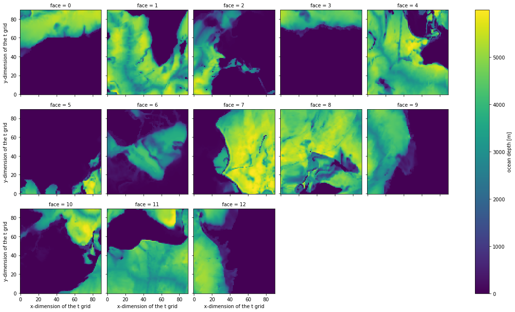
This view is not the most useful. It reflects how the data is arranged logically, rather than geographically.
A Pretty Map#
To make plotting easier, we can define a quick function to plot the data in a more geographically friendly way. Eventually these plotting functions may be provided by the gcmplots package: xecco/gcmplots. For now, it is easy enough to roll our own.
[5]:
from matplotlib import pyplot as plt
import cartopy as cart
import pyresample

class LLCMapper:

    def __init__(self, ds, dx=0.25, dy=0.25):
        # Extract LLC 2D coordinates
        lons_1d = ds.XC.values.ravel()
        lats_1d = ds.YC.values.ravel()

        # Define original grid
        self.orig_grid = pyresample.geometry.SwathDefinition(lons=lons_1d, lats=lats_1d)

        # Longitudes latitudes to which we will we interpolate
        lon_tmp = np.arange(-180, 180, dx) + dx/2
        lat_tmp = np.arange(-90, 90, dy) + dy/2

        # Define the lat lon points of the two parts.
        self.new_grid_lon, self.new_grid_lat = np.meshgrid(lon_tmp, lat_tmp)
        self.new_grid  = pyresample.geometry.GridDefinition(lons=self.new_grid_lon,
                                                            lats=self.new_grid_lat)

    def __call__(self, da, ax=None, projection=cart.crs.Robinson(), lon_0=-60, **plt_kwargs):

        assert set(da.dims) == set(['face', 'j', 'i']), "da must have dimensions ['face', 'j', 'i']"

        if ax is None:
            fig, ax = plt.subplots(figsize=(12, 6), subplot_kw={'projection': projection})
        else:
            m = plt.axes(projection=projection)

        field = pyresample.kd_tree.resample_nearest(self.orig_grid, da.values,
                                                    self.new_grid,
                                                    radius_of_influence=100000,
                                                    fill_value=None)

        vmax = plt_kwargs.pop('vmax', field.max())
        vmin = plt_kwargs.pop('vmin', field.min())


        x,y = self.new_grid_lon, self.new_grid_lat

        # Find index where data is splitted for mapping
        split_lon_idx = round(x.shape[1]/(360/(lon_0 if lon_0>0 else lon_0+360)))


        p = ax.pcolormesh(x[:,:split_lon_idx], y[:,:split_lon_idx], field[:,:split_lon_idx],
                         vmax=vmax, vmin=vmin, transform=cart.crs.PlateCarree(), zorder=1, **plt_kwargs)
        p = ax.pcolormesh(x[:,split_lon_idx:], y[:,split_lon_idx:], field[:,split_lon_idx:],
                         vmax=vmax, vmin=vmin, transform=cart.crs.PlateCarree(), zorder=2, **plt_kwargs)

        ax.add_feature(cart.feature.LAND, facecolor='0.5', zorder=3)
        label = ''
        if da.name is not None:
            label = da.name
        if 'units' in da.attrs:
            label += ' [%s]' % da.attrs['units']
        cb = plt.colorbar(p, shrink=0.4, label=label)
        return ax
[6]:
mapper = LLCMapper(coords)
mapper(coords.Depth);
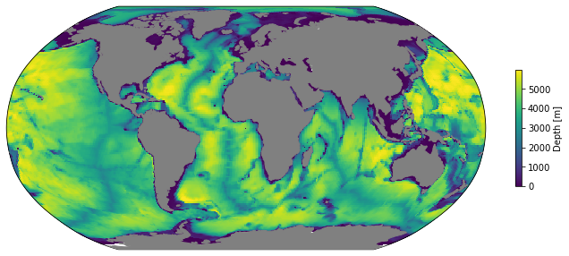
We can use this with any 2D cell-centered LLC variable.
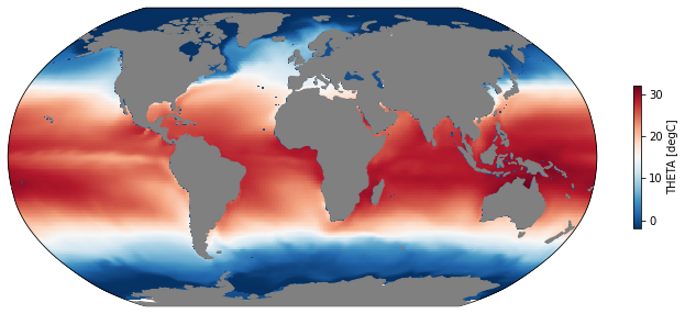
Selecting data#
The entire ECCOv4e3 dataset is contained in a single Xarray.Dataset object. How do we find a view specific pieces of data? This is handled by Xarray’s indexing and selecting functions. To get the SST from January 2000, we do this:
[7]:
sst = ds.THETA.sel(time='2000-01-15', k=0)
sst
[7]:
<xarray.DataArray 'THETA' (face: 13, j: 90, i: 90)>
dask.array<getitem, shape=(13, 90, 90), dtype=float32, chunksize=(13, 90, 90), chunktype=numpy.ndarray>
Coordinates:
  * face     (face) int64 0 1 2 3 4 5 6 7 8 9 10 11 12
  * i        (i) int64 0 1 2 3 4 5 6 7 8 9 10 ... 80 81 82 83 84 85 86 87 88 89
  * j        (j) int64 0 1 2 3 4 5 6 7 8 9 10 ... 80 81 82 83 84 85 86 87 88 89
    k        int64 0
    time     datetime64[ns] 2000-01-15
Attributes:
    long_name:      Potential Temperature
    standard_name:  THETA
units: degC- face: 13
- j: 90
- i: 90
- dask.array<chunksize=(13, 90, 90), meta=np.ndarray>
Array Chunk Bytes 421.20 kB 421.20 kB Shape (13, 90, 90) (13, 90, 90) Count 290 Tasks 1 Chunks Type float32 numpy.ndarray - face(face)int640 1 2 3 4 5 6 7 8 9 10 11 12
- standard_name :
- face_index
array([ 0, 1, 2, 3, 4, 5, 6, 7, 8, 9, 10, 11, 12])
- i(i)int640 1 2 3 4 5 6 ... 84 85 86 87 88 89
- axis :
- X
- long_name :
- x-dimension of the t grid
- standard_name :
- x_grid_index
- swap_dim :
- XC
array([ 0, 1, 2, 3, 4, 5, 6, 7, 8, 9, 10, 11, 12, 13, 14, 15, 16, 17, 18, 19, 20, 21, 22, 23, 24, 25, 26, 27, 28, 29, 30, 31, 32, 33, 34, 35, 36, 37, 38, 39, 40, 41, 42, 43, 44, 45, 46, 47, 48, 49, 50, 51, 52, 53, 54, 55, 56, 57, 58, 59, 60, 61, 62, 63, 64, 65, 66, 67, 68, 69, 70, 71, 72, 73, 74, 75, 76, 77, 78, 79, 80, 81, 82, 83, 84, 85, 86, 87, 88, 89]) - j(j)int640 1 2 3 4 5 6 ... 84 85 86 87 88 89
- axis :
- Y
- long_name :
- y-dimension of the t grid
- standard_name :
- y_grid_index
- swap_dim :
- YC
array([ 0, 1, 2, 3, 4, 5, 6, 7, 8, 9, 10, 11, 12, 13, 14, 15, 16, 17, 18, 19, 20, 21, 22, 23, 24, 25, 26, 27, 28, 29, 30, 31, 32, 33, 34, 35, 36, 37, 38, 39, 40, 41, 42, 43, 44, 45, 46, 47, 48, 49, 50, 51, 52, 53, 54, 55, 56, 57, 58, 59, 60, 61, 62, 63, 64, 65, 66, 67, 68, 69, 70, 71, 72, 73, 74, 75, 76, 77, 78, 79, 80, 81, 82, 83, 84, 85, 86, 87, 88, 89]) - k()int640
- axis :
- Z
- long_name :
- z-dimension of the t grid
- standard_name :
- z_grid_index
- swap_dim :
- Z
array(0)
- time()datetime64[ns]2000-01-15
- axis :
- T
- long_name :
- Time
- standard_name :
- time
array('2000-01-15T00:00:00.000000000', dtype='datetime64[ns]')
- long_name :
- Potential Temperature
- standard_name :
- THETA
- units :
- degC
Still no data has been actually downloaded. That doesn’t happen until we call .load() explicitly or try to make a plot.
[8]:
mapper(sst, cmap='RdBu_r');
/srv/conda/envs/notebook/lib/python3.8/site-packages/matplotlib/colors.py:576: RuntimeWarning: overflow encountered in multiply
  xa *= self.N
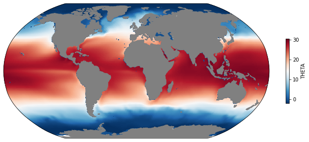
Do some Calculations#
Now let’s start doing something besides just plotting the existing data. For example, let’s calculate the time-mean SST.
[9]:
mean_sst = ds.THETA.sel(k=0).mean(dim='time')
mean_sst
[9]:
<xarray.DataArray 'THETA' (face: 13, j: 90, i: 90)>
dask.array<mean_agg-aggregate, shape=(13, 90, 90), dtype=float32, chunksize=(13, 90, 90), chunktype=numpy.ndarray>
Coordinates:
  * face     (face) int64 0 1 2 3 4 5 6 7 8 9 10 11 12
  * i        (i) int64 0 1 2 3 4 5 6 7 8 9 10 ... 80 81 82 83 84 85 86 87 88 89
  * j        (j) int64 0 1 2 3 4 5 6 7 8 9 10 ... 80 81 82 83 84 85 86 87 88 89
k int64 0- face: 13
- j: 90
- i: 90
- dask.array<chunksize=(13, 90, 90), meta=np.ndarray>
Array Chunk Bytes 421.20 kB 421.20 kB Shape (13, 90, 90) (13, 90, 90) Count 963 Tasks 1 Chunks Type float32 numpy.ndarray - face(face)int640 1 2 3 4 5 6 7 8 9 10 11 12
- standard_name :
- face_index
array([ 0, 1, 2, 3, 4, 5, 6, 7, 8, 9, 10, 11, 12])
- i(i)int640 1 2 3 4 5 6 ... 84 85 86 87 88 89
- axis :
- X
- long_name :
- x-dimension of the t grid
- standard_name :
- x_grid_index
- swap_dim :
- XC
array([ 0, 1, 2, 3, 4, 5, 6, 7, 8, 9, 10, 11, 12, 13, 14, 15, 16, 17, 18, 19, 20, 21, 22, 23, 24, 25, 26, 27, 28, 29, 30, 31, 32, 33, 34, 35, 36, 37, 38, 39, 40, 41, 42, 43, 44, 45, 46, 47, 48, 49, 50, 51, 52, 53, 54, 55, 56, 57, 58, 59, 60, 61, 62, 63, 64, 65, 66, 67, 68, 69, 70, 71, 72, 73, 74, 75, 76, 77, 78, 79, 80, 81, 82, 83, 84, 85, 86, 87, 88, 89]) - j(j)int640 1 2 3 4 5 6 ... 84 85 86 87 88 89
- axis :
- Y
- long_name :
- y-dimension of the t grid
- standard_name :
- y_grid_index
- swap_dim :
- YC
array([ 0, 1, 2, 3, 4, 5, 6, 7, 8, 9, 10, 11, 12, 13, 14, 15, 16, 17, 18, 19, 20, 21, 22, 23, 24, 25, 26, 27, 28, 29, 30, 31, 32, 33, 34, 35, 36, 37, 38, 39, 40, 41, 42, 43, 44, 45, 46, 47, 48, 49, 50, 51, 52, 53, 54, 55, 56, 57, 58, 59, 60, 61, 62, 63, 64, 65, 66, 67, 68, 69, 70, 71, 72, 73, 74, 75, 76, 77, 78, 79, 80, 81, 82, 83, 84, 85, 86, 87, 88, 89]) - k()int640
- axis :
- Z
- long_name :
- z-dimension of the t grid
- standard_name :
- z_grid_index
- swap_dim :
- Z
array(0)
As usual, no data was loaded. Instead, mean_sst is a symbolic representation of the data that needs to be pulled and the computations that need to be executed to produce the desired result. In this case, the 288 original chunks all need to be read from cloud storage. Dask coordinates this automatically for us. But it does take some time.
[10]:
%time mean_sst.load()
CPU times: user 18.9 s, sys: 1.76 s, total: 20.6 s
Wall time: 42.7 s
[10]:
<xarray.DataArray 'THETA' (face: 13, j: 90, i: 90)>
array([[[ 0.        ,  0.        ,  0.        , ...,  0.        ,
          0.        ,  0.        ],
        [ 0.        ,  0.        ,  0.        , ...,  0.        ,
          0.        ,  0.        ],
        [ 0.        ,  0.        ,  0.        , ...,  0.        ,
          0.        ,  0.        ],
        ...,
        [ 0.22906627,  0.20126666,  0.18094039, ...,  0.04199786,
          0.06655131,  0.09593879],
        [ 0.43254805,  0.42036152,  0.4126501 , ...,  0.20539196,
          0.24391538,  0.29138586],
        [ 0.6535146 ,  0.65845466,  0.65769684, ...,  0.37179062,
          0.42764866,  0.49818808]],

       [[ 0.87210137,  0.89154845,  0.88329524, ...,  0.52988845,
          0.60233873,  0.6977836 ],
        [ 1.0961676 ,  1.1175991 ,  1.0779033 , ...,  0.68887544,
          0.774091  ,  0.89128804],
        [ 1.3072966 ,  1.3048965 ,  1.2159245 , ...,  0.85709995,
          0.9489381 ,  1.0793763 ],
...
        [27.479395  , 27.666166  , 27.793968  , ...,  1.4822977 ,
          1.3396592 ,  1.190825  ],
        [27.444382  , 27.641308  , 27.776764  , ...,  1.3742981 ,
          1.2040414 ,  1.031747  ],
        [27.411293  , 27.615599  , 27.76121   , ...,  1.314467  ,
          1.1131614 ,  0.91215134]],

       [[ 4.6964245 ,  4.2194605 ,  3.719968  , ...,  0.        ,
          0.        ,  0.        ],
        [ 4.747999  ,  4.2700696 ,  3.7787225 , ...,  0.        ,
          0.        ,  0.        ],
        [ 4.754464  ,  4.278542  ,  3.7964838 , ...,  0.        ,
          0.        ,  0.        ],
        ...,
        [ 1.0251521 ,  0.82211953,  0.58778673, ...,  0.        ,
          0.        ,  0.        ],
        [ 0.85189605,  0.6512579 ,  0.43876594, ...,  0.        ,
          0.        ,  0.        ],
        [ 0.71174276,  0.5037161 ,  0.30439517, ...,  0.        ,
          0.        ,  0.        ]]], dtype=float32)
Coordinates:
  * face     (face) int64 0 1 2 3 4 5 6 7 8 9 10 11 12
  * i        (i) int64 0 1 2 3 4 5 6 7 8 9 10 ... 80 81 82 83 84 85 86 87 88 89
  * j        (j) int64 0 1 2 3 4 5 6 7 8 9 10 ... 80 81 82 83 84 85 86 87 88 89
k int64 0- face: 13
- j: 90
- i: 90
- 0.0 0.0 0.0 0.0 0.0 0.0 0.0 0.0 ... 0.0 0.0 0.0 0.0 0.0 0.0 0.0 0.0
array([[[ 0. , 0. , 0. , ..., 0. , 0. , 0. ], [ 0. , 0. , 0. , ..., 0. , 0. , 0. ], [ 0. , 0. , 0. , ..., 0. , 0. , 0. ], ..., [ 0.22906627, 0.20126666, 0.18094039, ..., 0.04199786, 0.06655131, 0.09593879], [ 0.43254805, 0.42036152, 0.4126501 , ..., 0.20539196, 0.24391538, 0.29138586], [ 0.6535146 , 0.65845466, 0.65769684, ..., 0.37179062, 0.42764866, 0.49818808]], [[ 0.87210137, 0.89154845, 0.88329524, ..., 0.52988845, 0.60233873, 0.6977836 ], [ 1.0961676 , 1.1175991 , 1.0779033 , ..., 0.68887544, 0.774091 , 0.89128804], [ 1.3072966 , 1.3048965 , 1.2159245 , ..., 0.85709995, 0.9489381 , 1.0793763 ], ... [27.479395 , 27.666166 , 27.793968 , ..., 1.4822977 , 1.3396592 , 1.190825 ], [27.444382 , 27.641308 , 27.776764 , ..., 1.3742981 , 1.2040414 , 1.031747 ], [27.411293 , 27.615599 , 27.76121 , ..., 1.314467 , 1.1131614 , 0.91215134]], [[ 4.6964245 , 4.2194605 , 3.719968 , ..., 0. , 0. , 0. ], [ 4.747999 , 4.2700696 , 3.7787225 , ..., 0. , 0. , 0. ], [ 4.754464 , 4.278542 , 3.7964838 , ..., 0. , 0. , 0. ], ..., [ 1.0251521 , 0.82211953, 0.58778673, ..., 0. , 0. , 0. ], [ 0.85189605, 0.6512579 , 0.43876594, ..., 0. , 0. , 0. ], [ 0.71174276, 0.5037161 , 0.30439517, ..., 0. , 0. , 0. ]]], dtype=float32) - face(face)int640 1 2 3 4 5 6 7 8 9 10 11 12
- standard_name :
- face_index
array([ 0, 1, 2, 3, 4, 5, 6, 7, 8, 9, 10, 11, 12])
- i(i)int640 1 2 3 4 5 6 ... 84 85 86 87 88 89
- axis :
- X
- long_name :
- x-dimension of the t grid
- standard_name :
- x_grid_index
- swap_dim :
- XC
array([ 0, 1, 2, 3, 4, 5, 6, 7, 8, 9, 10, 11, 12, 13, 14, 15, 16, 17, 18, 19, 20, 21, 22, 23, 24, 25, 26, 27, 28, 29, 30, 31, 32, 33, 34, 35, 36, 37, 38, 39, 40, 41, 42, 43, 44, 45, 46, 47, 48, 49, 50, 51, 52, 53, 54, 55, 56, 57, 58, 59, 60, 61, 62, 63, 64, 65, 66, 67, 68, 69, 70, 71, 72, 73, 74, 75, 76, 77, 78, 79, 80, 81, 82, 83, 84, 85, 86, 87, 88, 89]) - j(j)int640 1 2 3 4 5 6 ... 84 85 86 87 88 89
- axis :
- Y
- long_name :
- y-dimension of the t grid
- standard_name :
- y_grid_index
- swap_dim :
- YC
array([ 0, 1, 2, 3, 4, 5, 6, 7, 8, 9, 10, 11, 12, 13, 14, 15, 16, 17, 18, 19, 20, 21, 22, 23, 24, 25, 26, 27, 28, 29, 30, 31, 32, 33, 34, 35, 36, 37, 38, 39, 40, 41, 42, 43, 44, 45, 46, 47, 48, 49, 50, 51, 52, 53, 54, 55, 56, 57, 58, 59, 60, 61, 62, 63, 64, 65, 66, 67, 68, 69, 70, 71, 72, 73, 74, 75, 76, 77, 78, 79, 80, 81, 82, 83, 84, 85, 86, 87, 88, 89]) - k()int640
- axis :
- Z
- long_name :
- z-dimension of the t grid
- standard_name :
- z_grid_index
- swap_dim :
- Z
array(0)
[11]:
mapper(mean_sst, cmap='RdBu_r');
/srv/conda/envs/notebook/lib/python3.8/site-packages/matplotlib/colors.py:576: RuntimeWarning: overflow encountered in multiply
  xa *= self.N
Speeding things up with a Dask Cluster#
How can we speed things up? In general, the main bottleneck for this type of data analysis is the speed with which we can read the data. With cloud storage, the access is highly parallelizeable.
From a Pangeo environment, we can create a Dask cluster to spread the work out amongst many compute nodes. This works on both HPC and cloud. In the cloud, the compute nodes are provisioned on the fly and can be shut down as soon as we are done with our analysis.
The code below will create a cluster with up to five compute nodes. These will be ramped up and down based on demand. It can take a few minutes to provision our nodes.
[13]:
from dask_gateway import Gateway
from dask.distributed import Client

gateway = Gateway()
cluster = gateway.new_cluster()
cluster.adapt(minimum=1, maximum=5)
cluster
[14]:
# from dask_gateway import GatewayCluster
# from dask.distributed import Client
# cluster = GatewayCluster()
# cluster.scale(5)
# client = Client(cluster)
# cluster
Now we re-run the mean calculation. Note how the dashboard helps us visualize what the cluster is doing.
[15]:
%time ds.THETA.isel(k=0).mean(dim='time').load()
CPU times: user 19.3 s, sys: 1.71 s, total: 21 s
Wall time: 37.5 s
[15]:
<xarray.DataArray 'THETA' (face: 13, j: 90, i: 90)>
array([[[ 0.        ,  0.        ,  0.        , ...,  0.        ,
          0.        ,  0.        ],
        [ 0.        ,  0.        ,  0.        , ...,  0.        ,
          0.        ,  0.        ],
        [ 0.        ,  0.        ,  0.        , ...,  0.        ,
          0.        ,  0.        ],
        ...,
        [ 0.22906627,  0.20126666,  0.18094039, ...,  0.04199786,
          0.06655131,  0.09593879],
        [ 0.43254805,  0.42036152,  0.4126501 , ...,  0.20539196,
          0.24391538,  0.29138586],
        [ 0.6535146 ,  0.65845466,  0.65769684, ...,  0.37179062,
          0.42764866,  0.49818808]],

       [[ 0.87210137,  0.89154845,  0.88329524, ...,  0.52988845,
          0.60233873,  0.6977836 ],
        [ 1.0961676 ,  1.1175991 ,  1.0779033 , ...,  0.68887544,
          0.774091  ,  0.89128804],
        [ 1.3072966 ,  1.3048965 ,  1.2159245 , ...,  0.85709995,
          0.9489381 ,  1.0793763 ],
...
        [27.479395  , 27.666166  , 27.793968  , ...,  1.4822977 ,
          1.3396592 ,  1.190825  ],
        [27.444382  , 27.641308  , 27.776764  , ...,  1.3742981 ,
          1.2040414 ,  1.031747  ],
        [27.411293  , 27.615599  , 27.76121   , ...,  1.314467  ,
          1.1131614 ,  0.91215134]],

       [[ 4.6964245 ,  4.2194605 ,  3.719968  , ...,  0.        ,
          0.        ,  0.        ],
        [ 4.747999  ,  4.2700696 ,  3.7787225 , ...,  0.        ,
          0.        ,  0.        ],
        [ 4.754464  ,  4.278542  ,  3.7964838 , ...,  0.        ,
          0.        ,  0.        ],
        ...,
        [ 1.0251521 ,  0.82211953,  0.58778673, ...,  0.        ,
          0.        ,  0.        ],
        [ 0.85189605,  0.6512579 ,  0.43876594, ...,  0.        ,
          0.        ,  0.        ],
        [ 0.71174276,  0.5037161 ,  0.30439517, ...,  0.        ,
          0.        ,  0.        ]]], dtype=float32)
Coordinates:
  * face     (face) int64 0 1 2 3 4 5 6 7 8 9 10 11 12
  * i        (i) int64 0 1 2 3 4 5 6 7 8 9 10 ... 80 81 82 83 84 85 86 87 88 89
  * j        (j) int64 0 1 2 3 4 5 6 7 8 9 10 ... 80 81 82 83 84 85 86 87 88 89
k int64 0- face: 13
- j: 90
- i: 90
- 0.0 0.0 0.0 0.0 0.0 0.0 0.0 0.0 ... 0.0 0.0 0.0 0.0 0.0 0.0 0.0 0.0
array([[[ 0. , 0. , 0. , ..., 0. , 0. , 0. ], [ 0. , 0. , 0. , ..., 0. , 0. , 0. ], [ 0. , 0. , 0. , ..., 0. , 0. , 0. ], ..., [ 0.22906627, 0.20126666, 0.18094039, ..., 0.04199786, 0.06655131, 0.09593879], [ 0.43254805, 0.42036152, 0.4126501 , ..., 0.20539196, 0.24391538, 0.29138586], [ 0.6535146 , 0.65845466, 0.65769684, ..., 0.37179062, 0.42764866, 0.49818808]], [[ 0.87210137, 0.89154845, 0.88329524, ..., 0.52988845, 0.60233873, 0.6977836 ], [ 1.0961676 , 1.1175991 , 1.0779033 , ..., 0.68887544, 0.774091 , 0.89128804], [ 1.3072966 , 1.3048965 , 1.2159245 , ..., 0.85709995, 0.9489381 , 1.0793763 ], ... [27.479395 , 27.666166 , 27.793968 , ..., 1.4822977 , 1.3396592 , 1.190825 ], [27.444382 , 27.641308 , 27.776764 , ..., 1.3742981 , 1.2040414 , 1.031747 ], [27.411293 , 27.615599 , 27.76121 , ..., 1.314467 , 1.1131614 , 0.91215134]], [[ 4.6964245 , 4.2194605 , 3.719968 , ..., 0. , 0. , 0. ], [ 4.747999 , 4.2700696 , 3.7787225 , ..., 0. , 0. , 0. ], [ 4.754464 , 4.278542 , 3.7964838 , ..., 0. , 0. , 0. ], ..., [ 1.0251521 , 0.82211953, 0.58778673, ..., 0. , 0. , 0. ], [ 0.85189605, 0.6512579 , 0.43876594, ..., 0. , 0. , 0. ], [ 0.71174276, 0.5037161 , 0.30439517, ..., 0. , 0. , 0. ]]], dtype=float32) - face(face)int640 1 2 3 4 5 6 7 8 9 10 11 12
- standard_name :
- face_index
array([ 0, 1, 2, 3, 4, 5, 6, 7, 8, 9, 10, 11, 12])
- i(i)int640 1 2 3 4 5 6 ... 84 85 86 87 88 89
- axis :
- X
- long_name :
- x-dimension of the t grid
- standard_name :
- x_grid_index
- swap_dim :
- XC
array([ 0, 1, 2, 3, 4, 5, 6, 7, 8, 9, 10, 11, 12, 13, 14, 15, 16, 17, 18, 19, 20, 21, 22, 23, 24, 25, 26, 27, 28, 29, 30, 31, 32, 33, 34, 35, 36, 37, 38, 39, 40, 41, 42, 43, 44, 45, 46, 47, 48, 49, 50, 51, 52, 53, 54, 55, 56, 57, 58, 59, 60, 61, 62, 63, 64, 65, 66, 67, 68, 69, 70, 71, 72, 73, 74, 75, 76, 77, 78, 79, 80, 81, 82, 83, 84, 85, 86, 87, 88, 89]) - j(j)int640 1 2 3 4 5 6 ... 84 85 86 87 88 89
- axis :
- Y
- long_name :
- y-dimension of the t grid
- standard_name :
- y_grid_index
- swap_dim :
- YC
array([ 0, 1, 2, 3, 4, 5, 6, 7, 8, 9, 10, 11, 12, 13, 14, 15, 16, 17, 18, 19, 20, 21, 22, 23, 24, 25, 26, 27, 28, 29, 30, 31, 32, 33, 34, 35, 36, 37, 38, 39, 40, 41, 42, 43, 44, 45, 46, 47, 48, 49, 50, 51, 52, 53, 54, 55, 56, 57, 58, 59, 60, 61, 62, 63, 64, 65, 66, 67, 68, 69, 70, 71, 72, 73, 74, 75, 76, 77, 78, 79, 80, 81, 82, 83, 84, 85, 86, 87, 88, 89]) - k()int640
- axis :
- Z
- long_name :
- z-dimension of the t grid
- standard_name :
- z_grid_index
- swap_dim :
- Z
array(0)
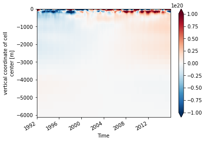
Spatially-Integrated Heat Content Anomaly#
Now let’s do something harder. We will calculate the horizontally integrated heat content anomaly for the full 3D model domain.
[16]:
# the monthly climatology
theta_clim = ds.THETA.groupby('time.month').mean(dim='time')
# the anomaly
theta_anom = ds.THETA.groupby('time.month') - theta_clim
rho0 = 1029
cp = 3994
ohc = rho0 * cp * (theta_anom *
                   coords.rA *
                   coords.hFacC).sum(dim=['face', 'j', 'i'])
ohc
[16]:
<xarray.DataArray (time: 288, k: 50)>
dask.array<mul, shape=(288, 50), dtype=float64, chunksize=(1, 50), chunktype=numpy.ndarray>
Coordinates:
  * k        (k) int64 0 1 2 3 4 5 6 7 8 9 10 ... 40 41 42 43 44 45 46 47 48 49
  * time     (time) datetime64[ns] 1992-01-15 1992-02-13 ... 2015-12-14
month (time) int64 1 2 3 4 5 6 7 8 9 10 11 ... 2 3 4 5 6 7 8 9 10 11 12- time: 288
- k: 50
- dask.array<chunksize=(1, 50), meta=np.ndarray>
Array Chunk Bytes 115.20 kB 400 B Shape (288, 50) (1, 50) Count 3895 Tasks 288 Chunks Type float64 numpy.ndarray - k(k)int640 1 2 3 4 5 6 ... 44 45 46 47 48 49
- axis :
- Z
- long_name :
- z-dimension of the t grid
- standard_name :
- z_grid_index
- swap_dim :
- Z
array([ 0, 1, 2, 3, 4, 5, 6, 7, 8, 9, 10, 11, 12, 13, 14, 15, 16, 17, 18, 19, 20, 21, 22, 23, 24, 25, 26, 27, 28, 29, 30, 31, 32, 33, 34, 35, 36, 37, 38, 39, 40, 41, 42, 43, 44, 45, 46, 47, 48, 49]) - time(time)datetime64[ns]1992-01-15 ... 2015-12-14
- axis :
- T
- long_name :
- Time
- standard_name :
- time
array(['1992-01-15T00:00:00.000000000', '1992-02-13T00:00:00.000000000', '1992-03-15T00:00:00.000000000', ..., '2015-10-15T00:00:00.000000000', '2015-11-14T00:00:00.000000000', '2015-12-14T00:00:00.000000000'], dtype='datetime64[ns]') - month(time)int641 2 3 4 5 6 7 ... 6 7 8 9 10 11 12
array([ 1,  2,  3,  4,  5,  6,  7,  8,  9, 10, 11, 12,  1,  2,  3,  4,  5,
        6,  7,  8,  9, 10, 11, 12,  1,  2,  3,  4,  5,  6,  7,  8,  9, 10,
       11, 12,  1,  2,  3,  4,  5,  6,  7,  8,  9, 10, 11, 12,  1,  2,  3,
        4,  5,  6,  7,  8,  9, 10, 11, 12,  1,  2,  3,  4,  5,  6,  7,  8,
        9, 10, 11, 12,  1,  2,  3,  4,  5,  6,  7,  8,  9, 10, 11, 12,  1,
        2,  3,  4,  5,  6,  7,  8,  9, 10, 11, 12,  1,  2,  3,  4,  5,  6,
        7,  8,  9, 10, 11, 12,  1,  2,  3,  4,  5,  6,  7,  8,  9, 10, 11,
       12,  1,  2,  3,  4,  5,  6,  7,  8,  9, 10, 11, 12,  1,  2,  3,  4,
        5,  6,  7,  8,  9, 10, 11, 12,  1,  2,  3,  4,  5,  6,  7,  8,  9,
       10, 11, 12,  1,  2,  3,  4,  5,  6,  7,  8,  9, 10, 11, 12,  1,  2,
        3,  4,  5,  6,  7,  8,  9, 10, 11, 12,  1,  2,  3,  4,  5,  6,  7,
        8,  9, 10, 11, 12,  1,  2,  3,  4,  5,  6,  7,  8,  9, 10, 11, 12,
        1,  2,  3,  4,  5,  6,  7,  8,  9, 10, 11, 12,  1,  2,  3,  4,  5,
        6,  7,  8,  9, 10, 11, 12,  1,  2,  3,  4,  5,  6,  7,  8,  9, 10,
       11, 12,  1,  2,  3,  4,  5,  6,  7,  8,  9, 10, 11, 12,  1,  2,  3,
        4,  5,  6,  7,  8,  9, 10, 11, 12,  1,  2,  3,  4,  5,  6,  7,  8,
        9, 10, 11, 12,  1,  2,  3,  4,  5,  6,  7,  8,  9, 10, 11, 12])
[17]:
# actually load the data
ohc.load()
# put the depth coordinate back for plotting purposes
ohc.coords['Z'] = coords.Z
ohc.swap_dims({'k': 'Z'}).transpose().plot(vmax=1e20)
[17]:
<matplotlib.collections.QuadMesh at 0x7f9c2d032610>
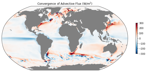
Spatial Derivatives: Heat Budget#
As our final exercise, we will do something much more complicated. We will compute the time-mean convergence of vertically-integrated heat fluxes. This is hard for several reasons.
The first reason it is hard is because it involves variables located at different grid points. Following MITgcm conventions, xmitgcm (which produced this dataset) labels the center point with the coordinates j, i, the u-velocity point as j, i_g, and the v-velocity point as j_g, i. The horizontal advective heat flux variables are
ADVx_TH    (time, k, face, j, i_g) float32 dask.array<shape=(288, 50, 13, 90, 90), chunksize=(1, 50, 13, 90, 90)>
ADVy_TH    (time, k, face, j_g, i) float32 dask.array<shape=(288, 50, 13, 90, 90), chunksize=(1, 50, 13, 90, 90)>
Xarray won’t allow us to add or multiply variables that have different dimensions, and xarray by itself doesn’t understand how to transform from one grid position to another.
That’s whyxgcmwas created.
Xgcm allows us to create a Grid object, which understands how to interpolate and take differences in a way that is compatible with finite volume models such at MITgcm. Xgcm also works with many other models, including ROMS, POP, MOM5/6, NEMO, etc.
A second reason this is hard is because of the complex topology connecting the different MITgcm faces. Fortunately xgcm also supports this.
[18]:
import xgcm

# define the connectivity between faces
face_connections = {'face':
                    {0: {'X':  ((12, 'Y', False), (3, 'X', False)),
                         'Y':  (None,             (1, 'Y', False))},
                     1: {'X':  ((11, 'Y', False), (4, 'X', False)),
                         'Y':  ((0, 'Y', False),  (2, 'Y', False))},
                     2: {'X':  ((10, 'Y', False), (5, 'X', False)),
                         'Y':  ((1, 'Y', False),  (6, 'X', False))},
                     3: {'X':  ((0, 'X', False),  (9, 'Y', False)),
                         'Y':  (None,             (4, 'Y', False))},
                     4: {'X':  ((1, 'X', False),  (8, 'Y', False)),
                         'Y':  ((3, 'Y', False),  (5, 'Y', False))},
                     5: {'X':  ((2, 'X', False),  (7, 'Y', False)),
                         'Y':  ((4, 'Y', False),  (6, 'Y', False))},
                     6: {'X':  ((2, 'Y', False),  (7, 'X', False)),
                         'Y':  ((5, 'Y', False),  (10, 'X', False))},
                     7: {'X':  ((6, 'X', False),  (8, 'X', False)),
                         'Y':  ((5, 'X', False),  (10, 'Y', False))},
                     8: {'X':  ((7, 'X', False),  (9, 'X', False)),
                         'Y':  ((4, 'X', False),  (11, 'Y', False))},
                     9: {'X':  ((8, 'X', False),  None),
                         'Y':  ((3, 'X', False),  (12, 'Y', False))},
                     10: {'X': ((6, 'Y', False),  (11, 'X', False)),
                          'Y': ((7, 'Y', False),  (2, 'X', False))},
                     11: {'X': ((10, 'X', False), (12, 'X', False)),
                          'Y': ((8, 'Y', False),  (1, 'X', False))},
                     12: {'X': ((11, 'X', False), None),
                          'Y': ((9, 'Y', False),  (0, 'X', False))}}}

# create the grid object
grid = xgcm.Grid(ds, periodic=False, face_connections=face_connections)
grid
[18]:
<xgcm.Grid>
X Axis (not periodic, boundary=None):
  * center   i --> left
  * left     i_g --> center
Y Axis (not periodic, boundary=None):
  * center   j --> left
  * left     j_g --> center
T Axis (not periodic, boundary=None):
  * center   time --> inner
  * inner    time_snp --> center
Z Axis (not periodic, boundary=None):
  * center   k --> left
  * left     k_l --> center
  * outer    k_p1 --> center
  * right    k_u --> center
Now we can use the grid object we created to take the divergence of a 2D vector
[19]:
# vertical integral and time mean of horizontal diffusive heat flux
advx_th_vint = ds.ADVx_TH.sum(dim='k').mean(dim='time')
advy_th_vint = ds.ADVy_TH.sum(dim='k').mean(dim='time')

# difference in the x and y directions
diff_ADV_th = grid.diff_2d_vector({'X': advx_th_vint, 'Y': advy_th_vint}, boundary='fill')
# convergence
conv_ADV_th = -diff_ADV_th['X'] - diff_ADV_th['Y']
conv_ADV_th
[19]:
<xarray.DataArray (face: 13, j: 90, i: 90)>
dask.array<sub, shape=(13, 90, 90), dtype=float32, chunksize=(1, 89, 89), chunktype=numpy.ndarray>
Coordinates:
  * face     (face) int64 0 1 2 3 4 5 6 7 8 9 10 11 12
  * j        (j) int64 0 1 2 3 4 5 6 7 8 9 10 ... 80 81 82 83 84 85 86 87 88 89
  * i        (i) int64 0 1 2 3 4 5 6 7 8 9 10 ... 80 81 82 83 84 85 86 87 88 89
- face: 13
- j: 90
- i: 90
- dask.array<chunksize=(1, 89, 89), meta=np.ndarray>
Array Chunk Bytes 421.20 kB 31.68 kB Shape (13, 90, 90) (1, 89, 89) Count 4311 Tasks 52 Chunks Type float32 numpy.ndarray - face(face)int640 1 2 3 4 5 6 7 8 9 10 11 12
- standard_name :
- face_index
array([ 0, 1, 2, 3, 4, 5, 6, 7, 8, 9, 10, 11, 12])
- j(j)int640 1 2 3 4 5 6 ... 84 85 86 87 88 89
- axis :
- Y
- long_name :
- y-dimension of the t grid
- standard_name :
- y_grid_index
- swap_dim :
- YC
array([ 0, 1, 2, 3, 4, 5, 6, 7, 8, 9, 10, 11, 12, 13, 14, 15, 16, 17, 18, 19, 20, 21, 22, 23, 24, 25, 26, 27, 28, 29, 30, 31, 32, 33, 34, 35, 36, 37, 38, 39, 40, 41, 42, 43, 44, 45, 46, 47, 48, 49, 50, 51, 52, 53, 54, 55, 56, 57, 58, 59, 60, 61, 62, 63, 64, 65, 66, 67, 68, 69, 70, 71, 72, 73, 74, 75, 76, 77, 78, 79, 80, 81, 82, 83, 84, 85, 86, 87, 88, 89]) - i(i)int640 1 2 3 4 5 6 ... 84 85 86 87 88 89
- axis :
- X
- long_name :
- x-dimension of the t grid
- standard_name :
- x_grid_index
- swap_dim :
- XC
array([ 0,  1,  2,  3,  4,  5,  6,  7,  8,  9, 10, 11, 12, 13, 14, 15, 16, 17,
       18, 19, 20, 21, 22, 23, 24, 25, 26, 27, 28, 29, 30, 31, 32, 33, 34, 35,
       36, 37, 38, 39, 40, 41, 42, 43, 44, 45, 46, 47, 48, 49, 50, 51, 52, 53,
       54, 55, 56, 57, 58, 59, 60, 61, 62, 63, 64, 65, 66, 67, 68, 69, 70, 71,
       72, 73, 74, 75, 76, 77, 78, 79, 80, 81, 82, 83, 84, 85, 86, 87, 88, 89])
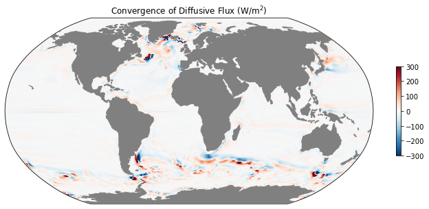
[20]:
# vertical integral and time mean of horizontal diffusive heat flux
difx_th_vint = ds.DFxE_TH.sum(dim='k').mean(dim='time')
dify_th_vint = ds.DFyE_TH.sum(dim='k').mean(dim='time')

# difference in the x and y directions
diff_DIF_th = grid.diff_2d_vector({'X': difx_th_vint, 'Y': dify_th_vint}, boundary='fill')
# convergence
conv_DIF_th = -diff_DIF_th['X'] - diff_DIF_th['Y']
conv_DIF_th
[20]:
<xarray.DataArray (face: 13, j: 90, i: 90)>
dask.array<sub, shape=(13, 90, 90), dtype=float32, chunksize=(1, 89, 89), chunktype=numpy.ndarray>
Coordinates:
  * face     (face) int64 0 1 2 3 4 5 6 7 8 9 10 11 12
  * j        (j) int64 0 1 2 3 4 5 6 7 8 9 10 ... 80 81 82 83 84 85 86 87 88 89
  * i        (i) int64 0 1 2 3 4 5 6 7 8 9 10 ... 80 81 82 83 84 85 86 87 88 89
- face: 13
- j: 90
- i: 90
- dask.array<chunksize=(1, 89, 89), meta=np.ndarray>
Array Chunk Bytes 421.20 kB 31.68 kB Shape (13, 90, 90) (1, 89, 89) Count 4311 Tasks 52 Chunks Type float32 numpy.ndarray - face(face)int640 1 2 3 4 5 6 7 8 9 10 11 12
- standard_name :
- face_index
array([ 0, 1, 2, 3, 4, 5, 6, 7, 8, 9, 10, 11, 12])
- j(j)int640 1 2 3 4 5 6 ... 84 85 86 87 88 89
- axis :
- Y
- long_name :
- y-dimension of the t grid
- standard_name :
- y_grid_index
- swap_dim :
- YC
array([ 0, 1, 2, 3, 4, 5, 6, 7, 8, 9, 10, 11, 12, 13, 14, 15, 16, 17, 18, 19, 20, 21, 22, 23, 24, 25, 26, 27, 28, 29, 30, 31, 32, 33, 34, 35, 36, 37, 38, 39, 40, 41, 42, 43, 44, 45, 46, 47, 48, 49, 50, 51, 52, 53, 54, 55, 56, 57, 58, 59, 60, 61, 62, 63, 64, 65, 66, 67, 68, 69, 70, 71, 72, 73, 74, 75, 76, 77, 78, 79, 80, 81, 82, 83, 84, 85, 86, 87, 88, 89]) - i(i)int640 1 2 3 4 5 6 ... 84 85 86 87 88 89
- axis :
- X
- long_name :
- x-dimension of the t grid
- standard_name :
- x_grid_index
- swap_dim :
- XC
array([ 0,  1,  2,  3,  4,  5,  6,  7,  8,  9, 10, 11, 12, 13, 14, 15, 16, 17,
       18, 19, 20, 21, 22, 23, 24, 25, 26, 27, 28, 29, 30, 31, 32, 33, 34, 35,
       36, 37, 38, 39, 40, 41, 42, 43, 44, 45, 46, 47, 48, 49, 50, 51, 52, 53,
       54, 55, 56, 57, 58, 59, 60, 61, 62, 63, 64, 65, 66, 67, 68, 69, 70, 71,
       72, 73, 74, 75, 76, 77, 78, 79, 80, 81, 82, 83, 84, 85, 86, 87, 88, 89])
[21]:
# convert to Watts / m^2 and load
mean_adv_conv = rho0 * cp * (conv_ADV_th/coords.rA).fillna(0.).load()
mean_dif_conv = rho0 * cp * (conv_DIF_th/coords.rA).fillna(0.).load()
/srv/conda/envs/notebook/lib/python3.8/site-packages/dask/core.py:121: RuntimeWarning: invalid value encountered in true_divide
  return func(*(_execute_task(a, cache) for a in args))
[22]:
ax = mapper(mean_adv_conv, cmap='RdBu_r', vmax=300, vmin=-300);
ax.set_title(r'Convergence of Advective Flux (W/m$^2$)');
[23]:
ax = mapper(mean_dif_conv, cmap='RdBu_r', vmax=300, vmin=-300)
ax.set_title(r'Convergence of Diffusive Flux (W/m$^2$)');
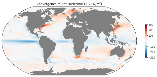
[24]:
ax = mapper(mean_dif_conv + mean_adv_conv, cmap='RdBu_r', vmax=300, vmin=-300)
ax.set_title(r'Convergence of Net Horizontal Flux (W/m$^2$)');
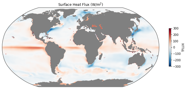
[25]:
ax = mapper(ds.TFLUX.mean(dim='time').load(), cmap='RdBu_r', vmax=300, vmin=-300);
ax.set_title(r'Surface Heat Flux (W/m$^2$)');
[ ]:
[ ]: